15 Time Series Inference
In the previous section, we considered time series regression models tailored for forecasting, where the regressors are based on past data relative to the dependent variable.
Of course, the regressors may also be contemporaneous as in the static time series regression Y_t = \alpha + \delta Z_t + u_t. The ADL model can also be extended by a contemporaneous exogenous variable: Y_t = \alpha_0 + \alpha_1 Y_{t-1} + \ldots + \alpha_p Y_{t-p} + \delta_0 Z_t + \delta_1 Z_{t-1} + \ldots + \delta_q Z_{t-q} + u_t.
Time series regressions have the general form Y_t = \boldsymbol X_t' \boldsymbol \beta + u_t, \quad t=1, \ldots, T. \qquad \quad \tag{15.1}
15.1 Assumptions for time series regression
Compared to cross-sectional regression, time series regressions require a stationarity condition instead of the i.i.d. assumption. Moreover, the error must be conditional mean independent of all past values, which indicates that the error represents the new information (shock) that was not available before time t. Variables that are conditional mean independent of the past are also called martingale difference sequence.
For the dynamic linear regression Equation 15.1 we make the following assumptions:
(A1-dyn) martingale difference sequence: E[u_t | \boldsymbol X_{t}, \boldsymbol X_{t-1}, \ldots] = 0.
(A2-dyn) stationary processes: \boldsymbol Z_t = (Y_t, \boldsymbol X_t')' is a stationary time series with the property that \boldsymbol Z_t and \boldsymbol Z_{t-\tau} become independent as \tau gets large.
(A3-dyn) large outliers unlikely: 0 < E[Y_{t}^4] < \infty, 0 < E[X_{tl}^4] < \infty for all l=1, \ldots, k.
(A4-dyn) no perfect multicollinearity: \boldsymbol X has full column rank.
The precise mathematical statement for “becoming independent as \tau gets large” is omitted here. It can be formulated with respect to a so-called strong mixing condition. It essentially requires that the dependency between \boldsymbol Z_t and \boldsymbol Z_{t-\tau} decrease as \tau \to \infty with a certain rate so that \boldsymbol Z_t and \boldsymbol Z_{t-\tau} are “almost independent” if \tau is large enough.
Under (A1-dyn)–(A4-dyn), the OLS estimator \widehat{\boldsymbol \beta} is consistent for \boldsymbol \beta and asymptotically normal.
15.2 Time series standard errors
We have \frac{\widehat \beta_l - \beta_l}{sd(\widehat \beta_l | \boldsymbol X)} \overset{D}{\to} \mathcal N(0,1) \quad \text{as} \ T \to \infty. The standard deviation sd(\widehat \beta_l | \boldsymbol X) is the squareroot of the (l,l)-entry of Var[\widehat{\boldsymbol \beta} | \boldsymbol X] = (\boldsymbol X' \boldsymbol X)^{-1} (\boldsymbol X' \boldsymbol D \boldsymbol X) (\boldsymbol X' \boldsymbol X)^{-1}, where \boldsymbol D = \boldsymbol Var[\boldsymbol u | \boldsymbol X].
If the errors are uncorrelated, i.e. Cov(u_t, u_{t-\tau}) = 0 for \tau \geq 1, the matrix \boldsymbol D is diagonal as in Section 5, and heteroskedasticity-consistent standard errors can be used. If the errors exhibit autocorrelation, then \boldsymbol D has an arbitrary form with off diagonal entries decaying slowly to zero as the distance to the main diagonal increases. In this case, heteroskedasticity and autorcorrelation-consistent (HAC) standard errors must be used.
You can check potential autocorrelation in the errors by consulting the ACF plot for the residuals:
data(gasoil, package="teachingdata2")
gas = zoo(diff(log(gasoil$gasoline)), gasoil$date)
oil = zoo(diff(log(gasoil$brent)), gasoil$date)
DL = dynlm(gas ~ L(oil, 1:2))
ADL = dynlm(gas ~ L(gas, 1:2) + L(oil, 1:2))
par(mfrow=c(1,2))
acf(DL$residuals, main="DL model")
acf(ADL$residuals, main = "ADL model")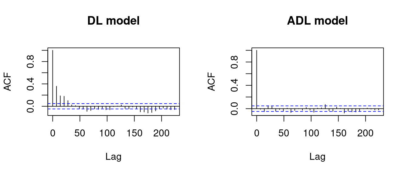
The residuals in the DL(2) model gas_t = \alpha + \delta_1 oil_{t-1} + \delta_2 oil_{t-2} + u_t indicate significant autocorrelation in the first few lags. The sample autocorrelations are above the blue dashed threshold.
The blue threshold indicates the critical value 1.96/\sqrt T for a test for the null hypothesis H_0: \rho(\tau) = 0.
We should use HAC standard errors:
coeftest(ADL, vcov. = vcovHC)
t test of coefficients:

               Estimate Std. Error t value  Pr(>|t|)
(Intercept)  0.00022028 0.00038647  0.5700   0.56877
L(gas, 1:2)1 0.37403773 0.06264798  5.9705 2.882e-09 ***
L(gas, 1:2)2 0.11072881 0.04516219  2.4518   0.01432 *
L(oil, 1:2)1 0.12355493 0.01020577 12.1064 < 2.2e-16 ***
L(oil, 1:2)2 0.00754501 0.01121716  0.6726   0.50127
---
Signif. codes:  0 '***' 0.001 '**' 0.01 '*' 0.05 '.' 0.1 ' ' 1
The residuals in the ADL(2,2) model gas_t = \alpha_0 + \alpha_1 gas_{t-1} + \alpha_2 gas_{t-2} + \delta_1 oil_{t-1} + \delta_2 oil_{t-2} + u_t indicate no autocorrelation in the error term. We can use HC standard errors:
coeftest(DL, vcov. = vcovHAC)
t test of coefficients:

               Estimate Std. Error t value  Pr(>|t|)
(Intercept)  0.00042119 0.00059160  0.7120    0.4766
L(oil, 1:2)1 0.17029082 0.01068906 15.9313 < 2.2e-16 ***
L(oil, 1:2)2 0.08437856 0.01128826  7.4749 1.239e-13 ***
---
Signif. codes:  0 '***' 0.001 '**' 0.01 '*' 0.05 '.' 0.1 ' ' 1
The following section highlights the importance of the variables being stationary in a time series regression.
15.3 Spurious correlation
Spurious correlation occurs when two unrelated time series Y_t and X_t have zero population correlation (Cov(Y_t, X_t) = 0) but exhibit a large sample correlation coefficient due to coincidental patterns or trends within the sample data.
Here are some examples of nonsense correlations: tylervigen.com/spurious-correlations.
Nonsense correlations may occur if the underlyung time series process is nonstationary.
15.3.1 Simulation evidence
Let’s simulate two independent AR(1) processes: Y_t = \alpha Y_{t-1} + u_t, \quad X_t = \alpha X_{t-1} + v_t, for t=1, \ldots, 200, where u_t and v_t are i.i.d. standard normal. If \alpha = 0.5, the processes are stationary. If \alpha = 1, the processes are nonstationary (random walk).
In any case, the population covariance is zero: Cov(Y_t, X_t) = 0. Therefore, we expect that the sample correlation is zero as well:
set.seed(121)
## Plot two independent AR(1) processes
u = rnorm(200)
v = rnorm(200)
Y1 = stats::filter(u, 0.5, "recursive")
X1 = stats::filter(v, 0.5, "recursive")
par(mfrow = c(1,2))
plot(Y1, main = "alpha = 0.5")
lines(X1, col="blue")
Y2 = stats::filter(u, 1, "recursive")
X2 = stats::filter(v, 1, "recursive")
plot(Y2, main = "alpha = 1")
lines(X2, col="blue")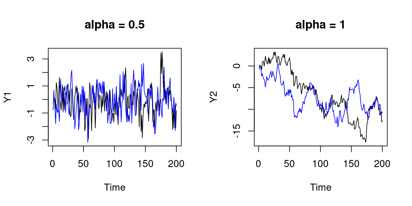
## Squared sample correlation for alpha = 0.5:
cor(Y1,X1)^2
[1] 0.0214327## Squared sample correlation for alpha = 1:
cor(Y2,X2)^2[1] 0.325291The squared sample correlation is equal to the R-squared of a simple regression of Y_t on X_t. The R-squared for the two independent stationary time series is close to zero, and the R-squared for the two independent nonstationary time series is unreasonably large.
The correlation of the differenced series is close to zero:
Of course, a large sample correlation of two uncorrelated series could occur by chance. Let’s repeat the simulation 10 times. Still, in many cases, the R-squared for the nonstationary series is much higher than expected:
## Simulate two independent AR(1) processes and R-squared
R2 = function(alpha, n=200){
  u = rnorm(n)
  v = rnorm(n)
  Y = stats::filter(u, alpha, "recursive")
  X = stats::filter(v, alpha, "recursive")
  return(cor(Y,X)^2)
}
## Get R-squared results with alpha = 0.5
c(R2(0.5, 200), R2(0.5, 200), R2(0.5, 200), R2(0.5, 200), R2(0.5, 200), R2(0.5, 200), R2(0.5, 200), R2(0.5, 200), R2(0.5, 200), R2(0.5, 200)) |> round(4)
[1] 0.0052 0.0038 0.0014 0.0081 0.0020 0.0044 0.0096 0.0187 0.0102 0.0190## Get R-squared results with alpha = 1
c(R2(1, 200), R2(1, 200), R2(1, 200), R2(1, 200), R2(1, 200), R2(1, 200), R2(1, 200), R2(1, 200), R2(1, 200), R2(1, 200)) |> round(4) [1] 0.0001 0.4746 0.3424 0.1782 0.4056 0.0385 0.1625 0.2406 0.3836 0.3570Increasing the sample size to T=1000 gives a similar picture:
c(R2(1, 1000), R2(1, 1000), R2(1, 1000), R2(1, 1000), R2(1, 1000), R2(1, 1000), R2(1, 1000), R2(1, 1000), R2(1, 1000), R2(1, 1000)) |> round(4) [1] 0.2365 0.0019 0.0215 0.4754 0.0425 0.2173 0.0030 0.4104 0.6846 0.3555The reason is that the OLS estimator is inconsistent if two independent random walks are regressed on each other. The key problem is that already simple moment statistics such as the sample mean or sample correlation are inconsistent for random walks. The behavior of the sample mean or OLS coefficients is driven by the stochastic path of the random walk.
Two completely unrelated random walks might share common upward and downward drifts by chance, which can produce high sample correlations although the population correlation is zero.
15.3.2 Real-world spurious correlations
The FRED-QD database offers a comprehensive collection of quarterly U.S. macroeconomic time series data. A subset of this data is contained in the package BVAR. See the appendix of this paper for a detailed description of the data.
We expect no relationship between the labor force participation rate and the Canada US exchange rate. However, the sample correlation coefficient is extremely high:
data(fred_qd, package = "BVAR")
par(mfrow=c(1,2))
plot(fred_qd$CIVPART, main="Labor force participation rate", type = "l")
plot(fred_qd$EXCAUSx, main="Canada US exchange rate", type = "l")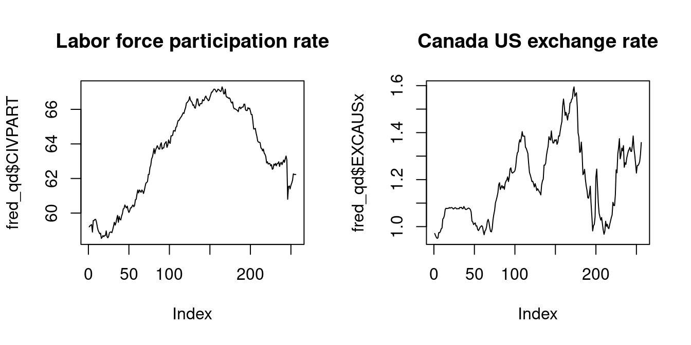
cor(fred_qd$CIVPART, fred_qd$EXCAUSx)[1] 0.648879plot(diff(fred_qd$CIVPART), main="Differenced CIVPART", type = "l")
plot(diff(fred_qd$EXCAUSx), main="Differenced EXCAUS", type = "l")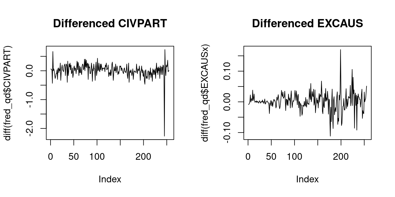
[1] -0.03030723The sample correlation of the differenced series indicates no relationship.
15.4 Testing for stationarity
The ACF plot provides a useful tool to decide whether a time series exhibits stationary or nonstationary behavior. We can also run a hypothesis test for the hypothesis that a series is nonstationary against the alternative that it is stationary.
15.4.1 Dickey Fuller test
Consider the AR(1) plus constant model: Y_t = c + \phi Y_{t-1} + u_t, \qquad \quad \tag{15.2} where u_t is an i.i.d. zero mean sequence.
Y_t is stationary if |\phi| < 1 and nonstationary if \phi = 1 (the cases \phi > 1 and \phi \leq -1 lead to exponential or oscillating behavior and are ignored here).
Let’s consider the hypotheses \underbrace{H_0: \phi = 1}_{\text{nonstationarity}} \quad vs. \quad \underbrace{H_1: |\phi| < 1}_{\text{stationarity}} To test H_0, we can run a t-test for \phi = 1. The t-statistic is Z_{\widehat \phi} = \frac{\widehat \phi - 1}{se(\widehat \phi)}, where \widehat \phi is the OLS estimator and se(\widehat \phi) is the homoskedasticity-only standard error.
Unfortunately, under H_0 the time series regression assumptions are not satisfied because Y_t is a random walk. The OLS estimator is not normally distributed, but is is consistent. It can be shown that the t-statistic does not converge to a standard normal distribution. Instead, it converges to the Dickey-Fuller distribution: Z_{\widehat \phi} \overset{D}{\longrightarrow} DF
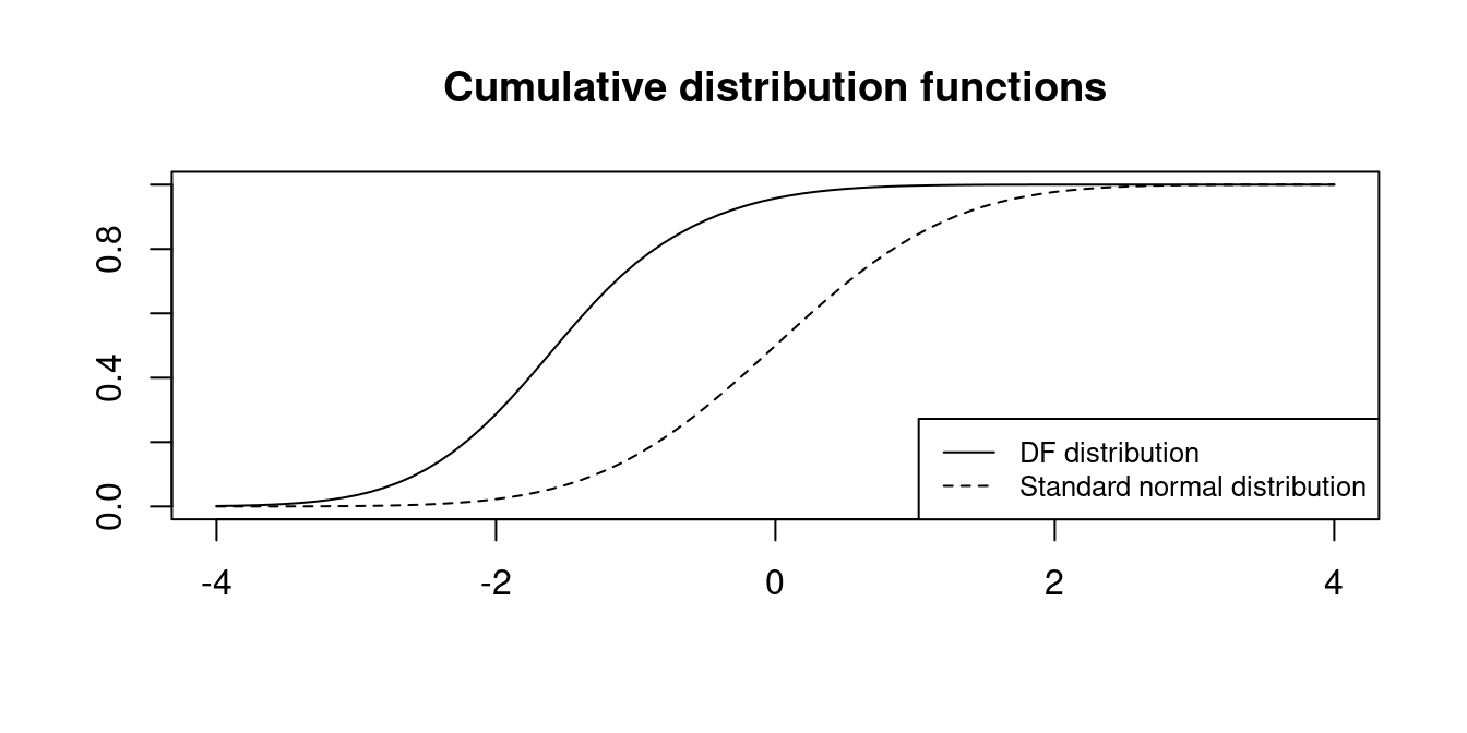
The critical values are much smaller:
| 0.01 | 0.025 | 0.05 | 0.1 | |
|---|---|---|---|---|
| \mathcal N(0,1) | -2.32 | -1.96 | -1.64 | -1.28 |
| DF | -3.43 | -3.12 | -2.86 | -2.57 |
More quantiles for the DF distribution can be obtained from the function qunitroot() from the urca package.
We reject H_0 if the t-statistic Z_{\widehat \phi} is smaller than the corresponding critical value from the above table.
15.4.2 Augmented Dickey Fuller test
The assumption that \Delta Y_t = Y_t - Y_{t-1} = u_t in Equation 15.2 is i.i.d. is unreasonable in many cases. It is more realistic that Y_t = c + \phi_1 Y_{t-1} + \ldots + \phi_p Y_{t-p} + u_t for some lag order p. In this model, Y_t is nonstationary if \sum_{j=1}^p \phi_j = 1.
The equation can be rewritten as \Delta Y_t = c + \psi Y_{t-1} + \theta_1 \Delta Y_{t-1} + \ldots + \theta_{p-1} \Delta Y_{t-(p-1)} + u_t, \qquad \quad \tag{15.3} where \psi = \sum_{j=1}^p \phi_j-1 and \theta_i = -\sum_{j=i+1}^p \phi_j.
To test for nonstationarity, we formulate the null hypothesis H_0: \sum_{j=1}^p \phi_j = 1, which is equivalent to H_0: \psi = 0.
The t-statistic Z_{\widehat \psi} from Equation 15.3 converges under H_0 to the DF distribution as well. Therefore, we can reject the null hypothesis of nonstationarity, if Z_{\widehat \psi} is smaller than the corresponding quantile from the DF distribution.
This test is called Augmented Dickey-Fuller test (ADF).
data(gdp, package="teachingdata")
data(gdpgr, package="teachingdata")
par(mfrow = c(2,2))
plot(gdp, main="Nominal GDP Germany")
plot(gdpgr, main = "Annual nominal GDP growth")
acf(gdp)
acf(gdpgr)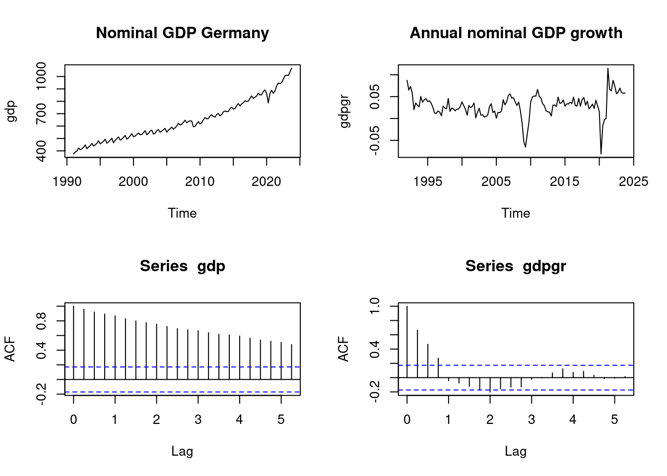
We use the ur.df() function from the urca package with the option type = "drift" to compute the ADF test statistic.
###############################################################
# Augmented Dickey-Fuller Test Unit Root / Cointegration Test #
###############################################################

The value of the test statistic is: 2.4235 7.8698
The ADF statistic Z_{\widehat \psi} is the fist value from the output. The critical value for \alpha = 0.05 is -2.86. Hence, the ADF with p = 4 does not reject the null hypothesis that GDP is nonstationary.
ur.df(gdpgr, type = "drift", lags = 4)
###############################################################
# Augmented Dickey-Fuller Test Unit Root / Cointegration Test #
###############################################################

The value of the test statistic is: -4.1546 8.6402
The ADF statistic with p = 4 is below -2.86, and the ADF test rejects the null hypothesis that GDP growth is nonstationary at the 5% significance level.
These results are in line with the observations from the ACF plots.