10 Case Study II: Drunk Driving
The dataset Fatalities contains panel data for traffic fatalities in the United States. Among others, it contains variables related to traffic fatalities and alcohol, including the number of traffic fatalities, the type of drunk driving laws and the tax on beer, reporting their values for each state and each year.
Here we will study how effective various government policies designed to discourage drunk driving actually are in reducing traffic deaths.
The measure of traffic deaths we use is the fatality rate, which is the annual number of traffic fatalities per 10000 individuals within the state’s population. The measure of alcohol taxes we use is the “real” tax on a case of beer, which is the beer tax, put into 1988 dollars by adjusting for inflation.
Let’s take a look at the structure of the dataset first.
str(Fatalities)We can see the data has been effectively defined as a data frame, with 336 observations of 34 variables. Our panel index variables are state (individual, i) and year (time, t).
It’s always good to have a quick look at the first few observations. The head() function in R, by default, shows the first six observations (rows) of a data frame or data set. However, you can specify a different number of rows to display by providing the desired count as an argument to the function if needed, like head(your_data_frame, n = 10) to display the first 10 rows.
     state       year
 al     :  7   1982:48
 az     :  7   1983:48
 ar     :  7   1984:48
 ca     :  7   1985:48
 co     :  7   1986:48
 ct     :  7   1987:48
 (Other):294   1988:48
Notice that the variable state is a factor variable with 48 levels (one for each of the 48 contiguous federal states of the U.S.). The variable year is also a factor variable that has 7 levels identifying the time period when the observation was made. This gives us 7×48=336 observations in total.
Since all variables are observed for all entities (states) and over all time periods, the panel is balanced. If there were missing data for at least one entity in at least one time period we would call the panel unbalanced.
10.1 Cross-sectional Regression
Let’s start by estimating simple regressions using data for years 1982 and 1988 that model the relationship between the beer tax (adjusted for 1988 dollars) and the traffic fatality rate, measured as the number of fatalities per 10000 inhabitants. Afterwards, we plot the data and add the corresponding estimated regression functions.
# define the fatality rate
Fatalities$fatal_rate = Fatalities$fatal / Fatalities$pop * 10000

# subset the data
Fatalities1982 = Fatalities |> subset(year == "1982")
Fatalities1988 = Fatalities |> subset(year == "1988")

# estimate simple regression models using 1982 and 1988 data
fatal1982_mod = lm(fatal_rate ~ beertax, data = Fatalities1982)
fatal1988_mod = lm(fatal_rate ~ beertax, data = Fatalities1988)

coeftest(fatal1982_mod, vcov. = vcovHC)
t test of coefficients:

            Estimate Std. Error t value Pr(>|t|)
(Intercept)  2.01038    0.15278 13.1586   <2e-16 ***
beertax      0.14846    0.14500  1.0238   0.3113
---
Signif. codes: 0 '***' 0.001 '**' 0.01 '*' 0.05 '.' 0.1 ' ' 1coeftest(fatal1988_mod, vcov. = vcovHC)
t test of coefficients:

            Estimate Std. Error t value  Pr(>|t|)
(Intercept)  1.85907    0.11786 15.7731 < 2.2e-16 ***
beertax      0.43875    0.14224  3.0847  0.003443 **
---
Signif. codes:  0 '***' 0.001 '**' 0.01 '*' 0.05 '.' 0.1 ' ' 1
The estimated regression functions are
\begin{align*} \widehat{FatalityRate} &= \underset{(0.15)}{2.01} + \underset{(0.15)}{0.15} \, BeerTax \quad (\text{1982 data}) \\ \widehat{FatalityRate} &= \underset{(0.12)}{1.86} + \underset{(0.14)}{0.44} \, BeerTax \quad (\text{1988 data}) \end{align*}
par(mfrow = c(1,2))
plot(fatal_rate~beertax, data = Fatalities1982,
     xlab = "Beer tax (in 1988 USD)", ylab = "Fatality rate (per 10000)",
     main = "1982", ylim = c(1, 4.2),
     pch = 20, col = "steelblue")
abline(fatal1982_mod, lwd = 1.5, col="darkred")
plot(fatal_rate~beertax, data = Fatalities1988,
     xlab = "Beer tax (in 1988 USD)", ylab = "Fatality rate (per 10000)",
     main = "1988", ylim = c(1, 4.2),
     pch = 20, col = "steelblue")
abline(fatal1988_mod, lwd = 1.5, col="darkred")
legend("bottomright",lty=1,col="darkred","Regression fit", cex = 0.8)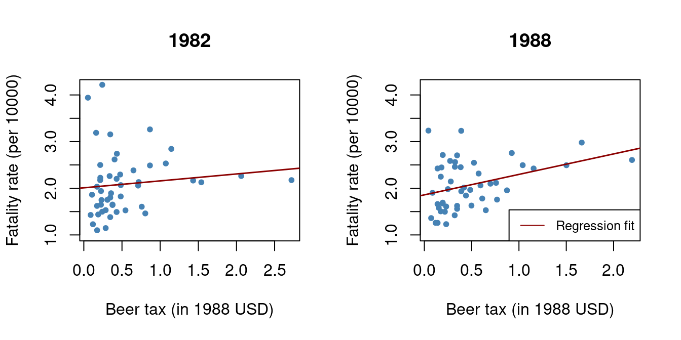
In both plots, each point represents observations of beer tax and fatality rate for a given state in the respective year. The regression results indicate a positive relationship between the beer tax and the fatality rate for both years.
The estimated coefficient on beer tax for the 1988 data is almost three times as large as for the 1982 dataset. This is contrary to our expectations: alcohol taxes are supposed to lower the rate of traffic fatalities. This is possibly due to omitted variable bias, since none of the models include any covariates, e.g., economic conditions.
Panel data methods could help here to account for omitted unobservable factors that vary from state to state but can be assumed to be constant over the observation period (e.g., attitudes toward drunk driving, road quality, density of cars on the road) and factors that vary from year to year but can be assumed to be constant for all states in a given year (e.g., changing national attitudes toward drunk driving, improvements in car safety over time).
10.2 “Before and After” Comparisons
Let’s suppose there are only T=2 time periods t=1982,1988. This allows us to analyze differences in changes of the fatality rate from year 1982 to 1988. We start by considering the population regression model:
\text{FatalityRate}_{it} = \beta_0 + \beta_1 \text{BeerTax}_{it} + \beta_2 Z_i + u_{it}
where the Z_i are state specific characteristics that differ between states but are constant over time. For t=1982 and t=1988 we have
\begin{align*} FatalityRate_{i,1982} = \beta_0 + \beta_1 \text{BeerTax}_{i,1982} + \beta_2 Z_i + u_{i,1982}, \\ FatalityRate_{i,1988} = \beta_0 + \beta_1 \text{BeerTax}_{i,1988} + \beta_2 Z_i + u_{i,1988}. \end{align*}
We can eliminate the Z_i by regressing the difference in the fatality rate between 1988 and 1982 on the difference in beer tax between those years:
\begin{align*} &\text{FatalityRate}_{i,1988} - \text{FatalityRate}_{i,1982} \\ &= \beta_1 (\text{BeerTax}_{i,1988} - \text{BeerTax}_{i,1982}) + u_{i,1988} - u_{i,1982} \end{align*}
This regression model, where the difference in fatality rate between 1988 and 1982 is regressed on the difference in beer tax between those years, yields an estimate for \beta_1 that is robust to a possible bias due to omission of Z_i, as these influences are eliminated from the model. Next we will estimate a regression based on the differenced data and plot the estimated regression function.
# compute the differences
diff_fatal_rate = Fatalities1988$fatal_rate - Fatalities1982$fatal_rate
diff_beertax = Fatalities1988$beertax - Fatalities1982$beertax

# estimate a regression using differenced data
fatal_diff_mod = lm(diff_fatal_rate ~ diff_beertax)
coeftest(fatal_diff_mod, vcov = vcovHC)
t test of coefficients:

              Estimate Std. Error t value Pr(>|t|)
(Intercept)  -0.072037   0.067854 -1.0616  0.29394
diff_beertax -1.040973   0.408288 -2.5496  0.01418 *
---
Signif. codes:  0 '***' 0.001 '**' 0.01 '*' 0.05 '.' 0.1 ' ' 1
Including the intercept allows for a change in the mean fatality rate in the time between 1982 and 1988 in the absence of a change in the beer tax.
We obtain the OLS estimated regression function
\begin{align*} &\widehat{FatalityRate_{i,1988} - FatalityRate_{i,1982}} \\ &= \underset{(-0.07)}{-0.072} - \underset{(0.41)}{1.04} \, (BeerTax_{i,1988} - BeerTax_{i,1982}) \end{align*}
plot(diff_fatal_rate ~ diff_beertax,
     xlab = "Change in beer tax (in 1988 USD)",
     ylab = "Change in fatality rate (per 10000)",
     main = "Changes in Traffic Fatality Rates and Beer Taxes in 1982-1988",
     ylim = c(-1.5, 1), cex.main=1,
     pch = 20, col = "steelblue")
abline(fatal_diff_mod, lwd = 1.5,col="darkred") # add the regression line to plot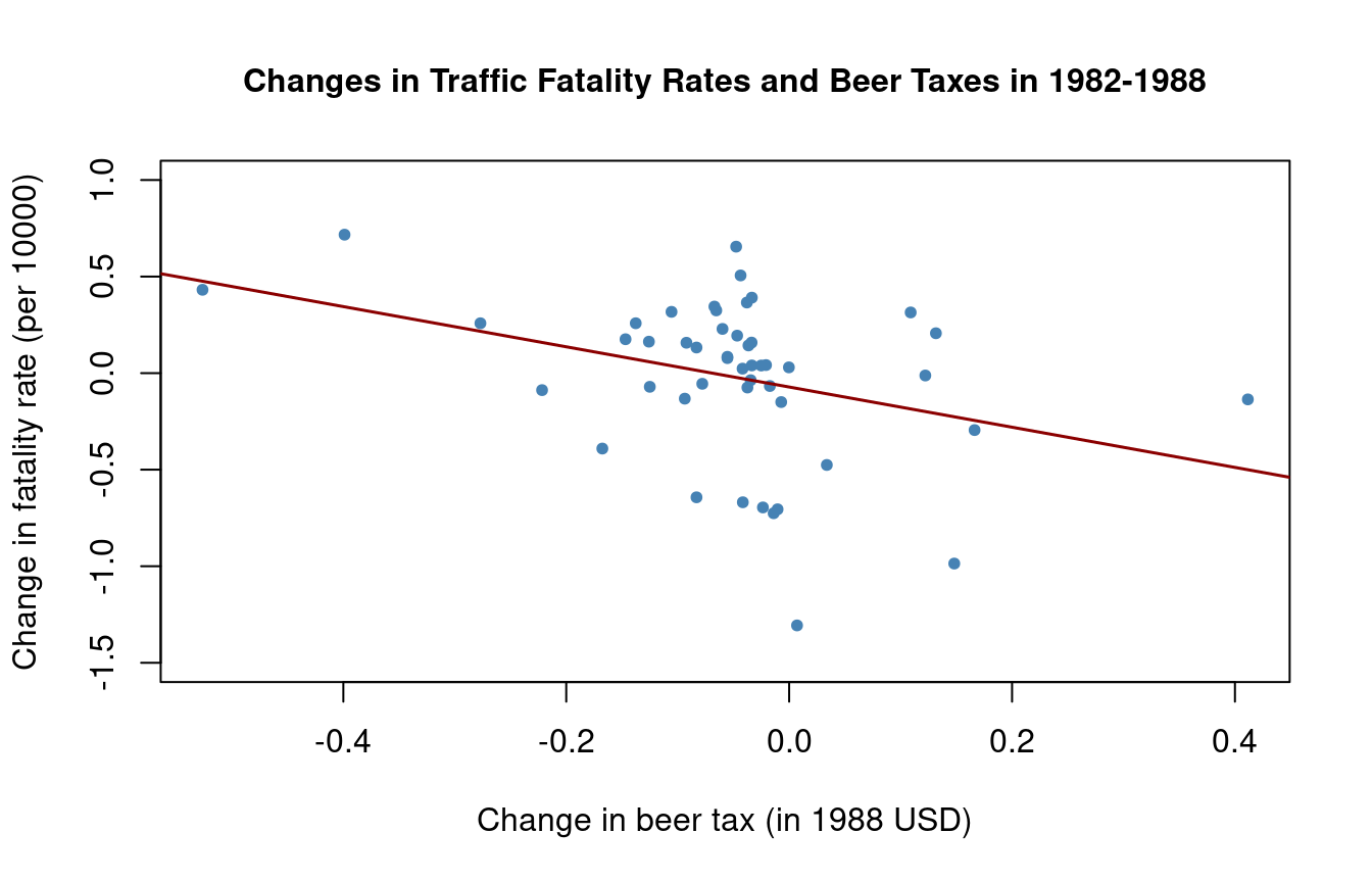
The estimated coefficient on beer tax is now negative and significantly different from zero at the 5\% significance level. Its interpretation is that raising the beer tax by \$1 is associated with an average decrease of 1.04 fatalities per 10000 inhabitants. This is rather large as the average fatality rate is approximately 2 persons per 10000 inhabitants.
# mean fatality rate over all states and time periods
mean(Fatalities$fatal_rate)
[1] 2.040444The outcome we obtained is likely to be a consequence of omitting factors in the single-year regression that influence the fatality rate and are correlated with the beer tax and change over time. The message is that we need to be more careful and control for such factors before drawing conclusions about the effect of a raise in beer taxes.
The approach presented in this section discards information for years 1983 to 1987. The fixed effects method allows us to use data for more than T=2 time periods and enables us to add control variables to the analysis.
10.3 State Fixed Effects
To estimate the relation between traffic fatality rates and beer taxes, the simple fixed effects model is
FatalityRate_{it} = \alpha_i + \beta_1 BeerTax_{it} + u_{it} \qquad \quad \tag{10.1}
a regression of the traffic fatality rate on beer tax and 48 binary regressors (one for each federal state). In this model, we are using a fixed effects approach to account for the effect of each federal state. \alpha_i represents the state fixed effect. Including a fixed effect for each state means that we’re estimating separate intercepts (or constant terms) for each state.
fatal_fe = plm(fatal_rate ~ beertax,
               index = c("state", "year"),
               effect = "individual",
               model = "within",
               data = Fatalities)
coeftest(fatal_fe, vcov. = vcovHC)
t test of coefficients:

        Estimate Std. Error t value Pr(>|t|)
beertax -0.65587    0.28837 -2.2744  0.02368 *
---
Signif. codes:  0 '***' 0.001 '**' 0.01 '*' 0.05 '.' 0.1 ' ' 1
The estimated coefficient is again −0.6559. The estimated regression function is
\widehat{FatalityRate} = \underset{(0.29)}{-0.66} \, BeerTax + StateFE \qquad \quad \tag{10.2}
The coefficient on BeerTax is negative and statistically significant at the 5\% level. Its interpretation is that states with a \$1 higher beer tax have, on average, 0.66 fewer traffic fatalities per 10000 people, given the same state-specific time-constant characteristics.
Although including state fixed effects eliminates the risk of bias due to omitted factors that vary across states but not over time, we suspect that there are other omitted variables that vary over time, making it difficult to interpret the coefficient as a causal effect.
If you prefer the lm() function, you can also use the following command:
The -1 term tells R to exclude the intercept term that it would normally include by default. By doing this, we’re essentially saying that we don’t want to estimate an overall intercept for the model because we are already capturing the state-specific effects. This is a common practice in fixed effects models to avoid multicollinearity between the state-specific intercepts and the predictors.
While fatal_fe_lm and fatal_fe return the same coefficient estimate, vcovHC(fatal_fe_lm) returns the HC3 heteroskedasticity-robust covariance matrix and vcovHC(fatal_fe) returns the cluster-robust covariance matrix. The reason is that fatal_fe_lm is an lm object and fatal_fe is a plm object. Cluster-robust standard errors should be preferred due to the autocorrelation structure within each cluster (state).
10.4 Year Fixed Effects
Controlling for variables that are constant across entities but vary over time can be done by including time fixed effects. If there are only time fixed effects, the fixed effects regression model becomes
Y_{it} = \lambda_t + \beta_1 X_{it} + u_{it}
In some applications it is meaningful to include both entity (state) and time fixed effects. The two-way fixed effects model is
Y_{it} = \alpha_i + \lambda_t + \beta_1 X_{it} + u_{it}
The combined model allows to eliminate bias from unobservables that change over time but are constant over entities and it controls for factors that differ across entities but are constant over time.
Let’s estimate the combined entity and time fixed effects model of the relation between fatalities and beer tax,
FatalityRate_{it} = \beta_1 BeerTax_{it} + StateFE_i + TimeFE_t + u_{it}
fatal_twoway = plm(fatal_rate ~ beertax,
               index = c("state", "year"),
               effect = "twoways",
               model = "within",
               data = Fatalities)
coeftest(fatal_twoway, vcov. = vcovHC)
t test of coefficients:

        Estimate Std. Error t value Pr(>|t|)
beertax -0.63998    0.34963 -1.8305  0.06824 .
---
Signif. codes:  0 '***' 0.001 '**' 0.01 '*' 0.05 '.' 0.1 ' ' 1
The estimated regression function is
\widehat{FatalityRate} = \underset{(0.35)}{-0.64} \, BeerTax + StateFE + TimeFE \tag{10.3}
The result is close to the estimated coefficient for the regression model including only entity fixed effects, which was -0.66. Unsurprisingly, the coefficient is less precisely estimated, as we observe a slightly higher cluster-robust standard error for this new coefficient of -0.64. Nevertheless, it is still significantly different from zero at the 10\% level.
We conclude that the estimated relationship between traffic fatalities and the real beer tax is not affected by omitted variable bias due to factors that are constant either over time or across states.
10.5 Driving Laws and Economic Conditions
There are two major sources of omitted variable bias that are not accounted for by all of the models of the relation between traffic fatalities and beer taxes that we have considered so far: economic conditions and driving laws.
Fortunately, Fatalities has data on state-specific legal drinking age (drinkage), punishment (jail, service) and various economic indicators like unemployment rate (unemp) and per capita income (income). We may use these covariates to extend the preceding analysis.
These covariates are defined as follows:
-
unemp: a numeric variable stating the state specific unemployment rate. -
log(income): the logarithm of real per capita income (in 1988 dollars). -
miles: the state average miles per driver. -
drinkage: the state specific minimum legal drinking age. -
drinkagec: a discretized version ofdrinkagethat classifies states into four categories of minimal drinking age; 18, 19, 20, 21 and older. R denotes this as[18,19),[19,20),[20,21)and[21,22]. These categories are included as dummy regressors where[21,22]is chosen as the reference category. -
punish: a dummy variable with levels yes and no that measures if drunk driving is severely punished by mandatory jail time or mandatory community service (first conviction).
First, we define some relevant variables to include in our following regression models:
Next, we estimate six regression models using plm().
# estimate six models
fat_mod1 = plm(fatal_rate ~ beertax,
               index = c("state", "year"),
               model = "pooling",
               data = Fatalities)

fat_mod2 = plm(fatal_rate ~ beertax,
               index = c("state", "year"),
               effect = "individual",
               model = "within",
               data = Fatalities)

fat_mod3 = plm(fatal_rate ~ beertax,
               index = c("state", "year"),
               effect = "twoways",
               model = "within",
               data = Fatalities)

fat_mod4 = plm(fatal_rate ~ beertax
               + drinkagec + punish + miles + unemp + log(income),
               index = c("state", "year"),
               effect = "twoways",
               model = "within",
               data = Fatalities)

fat_mod5 = plm(fatal_rate ~ beertax
               + drinkagec + punish + miles,
               index = c("state", "year"),
               effect = "twoways",
               model = "within",
               data = Fatalities)

fat_mod6 = plm(fatal_rate ~ beertax
               + drinkage + punish + miles + unemp + log(income),
               index = c("state", "year"),
               effect = "twoways",
               model = "within",
               data = Fatalities)
We use stargazer() to generate a comprehensive tabular presentation of the results.
stargazer(fat_mod1, fat_mod2, fat_mod3, fat_mod4, fat_mod5, fat_mod6,
          se = rob_se,
          type="html",
          omit.stat = c("f", "rsq", "adj.rsq"),
          add.lines=list(
            c("State FE","no","yes","yes","yes","yes","yes"),
            c("Year FE","no","no","yes","yes","yes","yes"),
            c("Clustered SE","yes","yes","yes","yes","yes","yes"))
)| Dependent variable: | ||||||
| fatal_rate | ||||||
| (1) | (2) | (3) | (4) | (5) | (6) | |
| beertax | 0.365*** | -0.656** | -0.640* | -0.445 | -0.690** | -0.456 |
| (0.118) | (0.288) | (0.350) | (0.288) | (0.342) | (0.298) | |
| drinkagec19 | -0.046 | -0.065 | ||||
| (0.057) | (0.064) | |||||
| drinkagec20 | 0.004 | -0.090 | ||||
| (0.065) | (0.075) | |||||
| drinkagec21 | -0.028 | 0.010 | ||||
| (0.068) | (0.080) | |||||
| drinkage | -0.002 | |||||
| (0.021) | ||||||
| punishyes | 0.038 | 0.085 | 0.039 | |||
| (0.100) | (0.108) | (0.100) | ||||
| miles | 0.00001 | 0.00002* | 0.00001 | |||
| (0.00001) | (0.00001) | (0.00001) | ||||
| unemp | -0.063*** | -0.063*** | ||||
| (0.013) | (0.013) | |||||
| log(income) | 1.816*** | 1.786*** | ||||
| (0.616) | (0.625) | |||||
| Constant | 1.853*** | |||||
| (0.117) | ||||||
| State FE | no | yes | yes | yes | yes | yes |
| Year FE | no | no | yes | yes | yes | yes |
| Clustered SE | yes | yes | yes | yes | yes | yes |
| Observations | 336 | 336 | 336 | 335 | 335 | 335 |
| Note: | p<0.1; p<0.05; p<0.01 | |||||
While columns 2 and 3 recap the results of the regressions of Equation 10.1 and Equation 10.2, column 1 presents an estimate of the coefficient of interest in the naive OLS regression of the fatality rate on beer tax without any fixed effects. There we obtain a positive estimate for the coefficient on beer tax that is likely to be upward biased.
The sign of the estimate changes as we extend the model by both entity and time fixed effects in models 2 and 3. Nonetheless, as discussed before, the magnitudes of both estimates may be too large.
The model specifications 4 to 6 include covariates that shall capture the effect of overall state economic conditions as well as the legal framework. Nevertheless, considering model 4 as the baseline specification including covariates, we observe four interesting results:
1. Including these covariates is not leading to a major reduction of the estimated effect of the beer tax. The coefficient is not significantly different from zero at the 10\% level, which means that it is considered imprecise.
2. According to this regression model, the minimum legal drinking age is not associated with an effect on traffic fatalities: none of the three dummy variables are significantly different from zero at any common level of significance. Moreover, an F-Test of the joint hypothesis that all three coefficients are zero does not reject the null hypothesis. The next code chunk shows how to test this hypothesis:
# test if legal drinking age has no explanatory power (Wald test)
linearHypothesis(fat_mod4,
                 c("drinkagec19", "drinkagec20", "drinkagec21"),
                 vcov. = vcovHC)
Linear hypothesis test
Hypothesis:
drinkagec19 = 0
drinkagec20 = 0
drinkagec21 = 0
Model 1: restricted model
Model 2: fatal_rate ~ beertax + drinkagec + punish + miles + unemp + log(income)
Note: Coefficient covariance matrix supplied.
Res.Df Df Chisq Pr(>Chisq)
1 276
2 273 3 1.1345 0.76883. There is no statistical evidence indicating an association between punishment for first offenders and drunk driving: the corresponding coefficient is not significant at the 10\% level.
4. The coefficients on the economic variables representing employment rate and income per capita indicate an statistically significant association between these and traffic fatalities. We can check that the employment rate and income per capita coefficients are jointly significant at the 0.1\% level.
# test if economic indicators have no explanatory power
linearHypothesis(fat_mod4,
                 c("log(income)", "unemp"),
                 vcov. = vcovHC)
Linear hypothesis test
Hypothesis:
log(income) = 0
unemp = 0
Model 1: restricted model
Model 2: fatal_rate ~ beertax + drinkagec + punish + miles + unemp + log(income)
Note: Coefficient covariance matrix supplied.
Res.Df Df Chisq Pr(>Chisq)
1 275
2 273 2 63.155 1.932e-14 ***
---
Signif. codes: 0 '***' 0.001 '**' 0.01 '*' 0.05 '.' 0.1 ' ' 1Model 5 omits the economic factors. The result supports the notion that economic indicators should remain in the model as the coefficient on beer tax is sensitive to the inclusion of the latter.
Results for model 6 show that the legal drinking age has little explanatory power and that the coefficient of interest is not sensitive to changes in the functional form of the relation between drinking age and traffic fatalities.
10.6 Summary
We have not found statistical evidence to state that severe punishments and an increase in the minimum drinking age could lead to a reduction of traffic fatalities due to drunk driving.
Nonetheless, there seems to be a negative effect of alcohol taxes on traffic fatalities according to our model estimate. However, this estimate is not precise and cannot be interpreted as the causal effect of interest, as there still may be a bias.
There may be omitted variables that differ across states and change over time, and this bias remains even though we use a panel approach that controls for entity specific and time invariant unobservables.