lm(wage ~ education, data = cps)
Call:
lm(formula = wage ~ education, data = cps)

Coefficients:
(Intercept)    education
-16.448 2.898 The previous section discussed OLS regression from a descriptive perspective. A regression model puts the regression problem into a stochastic framework.
Let \{(Y_i, \boldsymbol X_i'), i=1, \ldots, n \} be a sample from some joint population distribution, where Y_i is individual i’s dependent variable, and \boldsymbol X_i = (1, X_{i2}, \ldots, X_{ik})' is the k \times 1 vector of individual i’s regressor variables.
Linear Regression Model
The linear regression model equation for individual i=1, \ldots, n is Y_i = \beta_1 + \beta_2 X_{i2} + \ldots + \beta_k X_{ik} + u_i where \boldsymbol \beta = (\beta_1, \ldots, \beta_k)' is the k \times 1 vector of regression coefficients and u_i is the error term for individual i. In vector notation, we write Y_i = \boldsymbol X_i' \boldsymbol \beta + u_i, \quad i=1, \ldots, n. \tag{4.1}
The error term represents further factors that affect the dependent variable and are not included in the model. These factors include measurement error, omitted variables, or unobserved/unmeasured variables.
The expression m(\boldsymbol X_i) = \boldsymbol X_i' \boldsymbol \beta is called the population regression function.
We can use matrix notation to describe the n individual regression equations together. Consider the n \times 1 dependent variable vector \boldsymbol Y, the n \times k regressor matrix \boldsymbol X, and the vectors of coefficients and error terms given by \underset{(k\times 1)}{\boldsymbol \beta} = \begin{pmatrix} \beta_1 \\ \vdots \\ \beta_k \end{pmatrix}, \quad \underset{(n\times 1)}{\boldsymbol u} = \begin{pmatrix} u_1 \\ \vdots \\ u_n \end{pmatrix}. The n equations of Equation 4.1 can be written together as \boldsymbol Y = \boldsymbol X \boldsymbol \beta + \boldsymbol u.
We assume that (Y_i, \boldsymbol X_i'), i=1, \ldots, n, satisfies Equation 4.1 with
(A1) conditional mean independence: E[u_i | \boldsymbol X_i] = 0
(A2) random sampling: (Y_i, \boldsymbol X_i') are i.i.d. draws from their joint population distribution
(A3) large outliers unlikely: 0 < E[Y_i^4] < \infty, 0 < E[X_{il}^4] < \infty for all l=1, \ldots, k
(A4) no perfect multicollinearity: \boldsymbol X has full column rank
optional: (A5) homoskedasticity: Var[u_i | \boldsymbol X_i] = \sigma^2
optional: (A6) normal errors: u_i | \boldsymbol X_i is normally distributed
Assumptions (A1)–(A4) are required and (A5) and (A6) are optional. Model (A1)–(A4) is called heteroskedastic linear regression model, model (A1)–(A5) is called homoskedastic linear regression model, and model (A1)–(A6) is called normal linear regression model.
(A1)–(A2) define the properties of the regression model, (A3)–(A4) imply that OLS can be used to estimate the model, and (A5)–(A6) ensure that classical exact inference can be used without relying on robust large sample methods.
For all i,j=1, \ldots, n, the model has the following properties:
Conditional expectation: (A1) implies E[Y_i | \boldsymbol X_i] = \boldsymbol X_i' \boldsymbol \beta = m(\boldsymbol X_i).
Weak exogeneity: (A1) implies E[u_i] = 0, \quad Cov(u_i, X_{il}) = 0.
Strict exogeneity: (A1)+(A2) imply E[u_i | \boldsymbol X] = 0, \quad Cov(u_i, X_{jl}) = 0.
Heteroskedasticity: (A1)+(A2) imply Var[u_i | \boldsymbol X] = E[u_i^2 | \boldsymbol X_i] =: \sigma_i^2
No autocorrelation: (A1)+(A2) imply E[u_i u_j | \boldsymbol X] = 0, \quad Cov(u_i, u_j) = 0, \quad i \neq j. The errors have a diagonal conditional covariance matrix: \boldsymbol D := Var[\boldsymbol u | \boldsymbol X] = \begin{pmatrix} \sigma_1^2 & 0 & \ldots & 0 \\ 0 & \sigma_2^2 & \ldots & 0 \\ \vdots & \vdots & \ddots & \vdots \\ 0 & 0 & \ldots & \sigma_n^2 \end{pmatrix}.
The OLS coefficient vector \widehat{\boldsymbol \beta} = (\boldsymbol X' \boldsymbol X)^{-1} \boldsymbol X' \boldsymbol Y can be used to estimate \boldsymbol \beta. For all i=1, \ldots, n and l=1, \ldots, K, the OLS estimator has the following properties:
Existence: (A4) implies that \boldsymbol X' \boldsymbol X is invertible and that \widehat{\boldsymbol \beta} exists.
Unbiasedness: (A1)+(A2)+(A4) imply E[\widehat{\boldsymbol \beta} | \boldsymbol X] = \boldsymbol \beta.
Sampling variance: (A1)+(A2)+(A4) imply Var[\widehat{\boldsymbol \beta} | \boldsymbol X] = (\boldsymbol X' \boldsymbol X)^{-1} (\boldsymbol X' \boldsymbol D \boldsymbol X) (\boldsymbol X' \boldsymbol X)^{-1}. If (A5) holds as well, then \boldsymbol D = \boldsymbol I_n and Var[\widehat{\boldsymbol \beta} | \boldsymbol X] = \sigma^2 (\boldsymbol X' \boldsymbol X)^{-1}.
Normality: (A1)+(A2)+(A4)+(A6) imply \widehat{\boldsymbol \beta} | \boldsymbol X \sim \mathcal N\Big(\boldsymbol \beta, Var[\widehat{\boldsymbol \beta} | \boldsymbol X] \Big)
Consistency: (A1)–(A4) imply \widehat{\boldsymbol \beta} \overset{p}{\rightarrow} \boldsymbol \beta\quad \text{as} \ n \to \infty since the bias is zero and the variance asymptotically tends to zero.
Asymptotic variance: Let \boldsymbol Q := E[\boldsymbol X_i \boldsymbol X_i'] and \boldsymbol \Omega := E[u_i^2 \boldsymbol X_i \boldsymbol X_i']. (A1)–(A4) imply Var[\widehat{ \boldsymbol \beta} | \boldsymbol X] = \underbrace{\frac{1}{n}}_{\to 0} \Big( \underbrace{\frac{1}{n} \boldsymbol X' \boldsymbol X}_{\overset{p}{\rightarrow} \boldsymbol Q} \Big)^{-1} \Big(\underbrace{\frac{1}{n} \boldsymbol X' \boldsymbol D \boldsymbol X}_{\overset{p}{\rightarrow} \boldsymbol \Omega} \Big) \Big( \underbrace{\frac{1}{n} \boldsymbol X' \boldsymbol X}_{\overset{p}{\rightarrow} \boldsymbol Q} \Big)^{-1} \overset{p}{\to} \boldsymbol 0, and Var[\sqrt n(\widehat{\boldsymbol \beta} - \boldsymbol \beta) | \boldsymbol X] \overset{p}{\to} \boldsymbol Q^{-1} \boldsymbol \Omega \boldsymbol Q^{-1}. If (A5) holds as well, then \boldsymbol \Omega = \sigma^2 \boldsymbol Q, and \boldsymbol Q^{-1} \boldsymbol \Omega \boldsymbol Q^{-1} = \sigma^2 \boldsymbol Q^{-1}.
Asymptotic normality: (A1)–(A4) imply \sqrt n (\widehat{\boldsymbol \beta} - \boldsymbol \beta) \overset{D}{\rightarrow} \mathcal N(\boldsymbol 0, \boldsymbol Q^{-1} \boldsymbol \Omega \boldsymbol Q^{-1}).
Technical details can be found in Appendix A.
For example, consider the regression model of hourly wage on education (years of schooling):
wage_i = \beta_1 + \beta_2 \ edu_i + u_i, \quad E[u_i | edu_i] = 0, \quad i=1, \ldots, n. \tag{4.2}
The population regression function is m(edu_i) = \beta_1 + \beta_2 edu_i. (A1) implies that E[wage_i | edu_i] = \underbrace{\beta_1 + \beta_2 edu_i}_{= m(edu_i)} + \underbrace{E[u_i | edu_i]}_{=0}. The average wage level of all individuals with z years of schooling is \beta_1 + \beta_2 z. Cov(wage_i, edu_i) = \underbrace{Cov(m(edu_i), edu_i)}_{= \beta_2 Var[edu_i]} + \underbrace{Cov(u_i, edu_i)}_{=0} The coefficient \beta_2 is identified as \beta_2 = \frac{Cov(wage_i, edu_i)}{Var[edu_i]} = Corr(wage_i, edu_i) \cdot \frac{sd(wage_i)}{sd(edu_i)}. The coefficient describes the correlative relationship between education and wages.
The marginal effect of education is \frac{\partial E[wage_i | edu_i]}{\partial edu_i} = \beta_2.
lm(wage ~ education, data = cps)
Call:
lm(formula = wage ~ education, data = cps)
Coefficients:
(Intercept) education
-16.448 2.898 Interpretation: People with one more year of education are paid on average 2.90 USD more than people with one year less of education.
The marginal effect is a correlative effect and does not say where exactly a higher wage level for people with more education comes from. Regression relationships do not necessarily imply a causal relationship.
People with more education may earn more for a number of reasons. Maybe they are generally smarter or come from wealthier families, which leads to better paying jobs. Or maybe more education actually leads to higher earning
The coefficient \beta_2 is a measure of how strongly education and earnings are correlated.
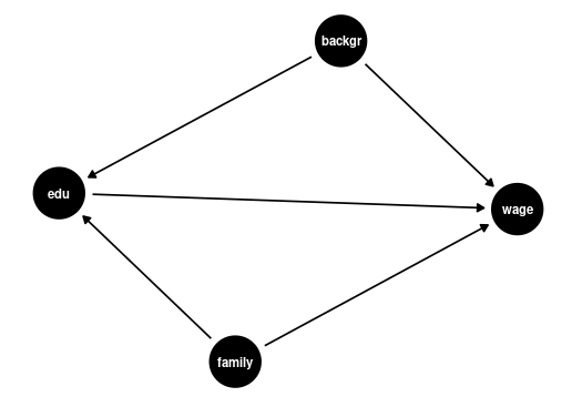
This association could be due to other factors that correlate with both wages and education, such as family background (parental education, family income, ethnicity, structural racism) or personal background (gender, intelligence).
Notice: Correlation does not imply causation!
To disentangle the causal effect of education on wages from other correlative effects, we can include control variables.
To understand the causal effect of an additional year of education on wages, it is crucial to consider the influence of family and personal background. These factors, if not included in our analysis, are known as omitted variables. An omitted variable is one that:
The presence of omitted variables means that we cannot be sure that the regression relationship between education and wages is purely causal. We say that we have omitted variable bias for the causal effect of the regressor of interest.
The coefficient \beta_2 in Equation 4.2 measures the correlative or marginal effect, not the causal effect. This must always be kept in mind when interpreting regression coefficients.
We can include control variables in the linear regression model to reduce omitted variable bias so that we can interpret \beta_2 as a ceteris paribus marginal effect (ceteris paribus means holding other variables constant).
For example, let’s include years of experience as well as racial background and gender dummy variables for Black and female: wage_i = \beta_1 + \beta_2 edu_i +\beta_3 ex_i + \beta_4 Black_i + \beta_5 fem_i + u_i. In this case, \beta_2 = \frac{\partial E[wage_i | edu_i, ex_i, Black_i, fem_i]}{\partial edu_i} is the marginal effect of education on expected wages, holding experience, race, and gender fixed.
lm(wage ~ education + experience + black + female, data = cps)
Call:
lm(formula = wage ~ education + experience + black + female,
    data = cps)

Coefficients:
(Intercept)    education   experience        black       female
   -21.7095       3.1350       0.2443      -2.8554      -7.4363
Interpretation: Given the same experience, racial background, and gender, people with one more year of education are paid on average 3.14 USD more than people with one year less of education.
Note: It does not hold other unobservable characteristics (such as ability) or variables not included in the regression (such as quality of education) fixed, so an omitted variable bias may still be present.
Good control variables are variables that are determined before the level of education is determined. Control variables should not be the cause of the dependent variable of interest.
Examples of good controls for education are parental education level, region of residence, or educational industry/field of study.
A problematic situation is when the control variable is the cause of education. Bad controls are typically highly correlated with the independent variable of interest and irrelevant to the causal effect of that variable on the dependent variable.
Examples of bad controls for education are current job position, number of professional certifications obtained, or number of job offers.
A high correlation of the bad control with the variable education also causes a high variance of the OLS coefficient for education and leads to an imprecise coefficient estimate. This problem is called imperfect multicollinearity.
Bad controls make it difficult to interpret causal relationships. They may control away the effect you want to measure, or they may introduce additional reverse causal effects hidden in the regression coefficients.
A linear dependence on wages and experience is a strong assumption. We can reasonably expect a nonlinear marginal effect of another year of experience on wages. For example, the effect may be higher for workers with 5 years of experience than for those with 40 years of experience.
Polynomials can be used to specify a nonlinear regression function: wage_i = \beta_1 + \beta_2 ex_i + \beta_3 ex_i^2 + \beta_4 ex_i^3 + u_i.
## we focus on Asian people only for illustration
cps.as = cps |> subset(asian == 1)
fit = lm(wage ~ experience + I(experience^2) + I(experience^3),
         data = cps.as)
coefficients(fit)
(Intercept) experience I(experience^2) I(experience^3)
20.4547146896 1.2013241316 -0.0446897909 0.0003937551 plot(wage ~ experience, data = cps.as, ylim = c(0,100))
lines(sort(cps.as$experience),
fitted(fit)[order(cps.as$experience)],
col='red', type='l', lwd=3) 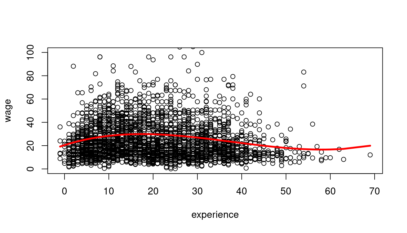
The marginal effect depends on the years of experience: \frac{\partial E[wage_i | ex_i] }{\partial ex_i} = \beta_2 + 2 \beta_3 ex_i + 3 \beta_4 exp_i^2. For instance, the additional wage for a worker with 11 years of experience compared to a worker with 10 years of experience is on average 1.43 + 2\cdot (-0.042) \cdot 10 + 3 \cdot 0.0003 \cdot 10^2 = 0.68.
A linear regression with interaction terms: wage_i = \beta_1 + \beta_2 edu_i + \beta_3 fem_i + \beta_4 marr_i + \beta_5 (marr_i \cdot fem_i) + u_i
lm(wage ~ education + female + married + married:female, data = cps)
Call:
lm(formula = wage ~ education + female + married + married:female,
    data = cps)

Coefficients:
   (Intercept)       education          female         married  female:married
       -17.886           2.867          -3.266           7.167          -5.767
The marginal effect of gender depends on the person’s marital status: \frac{\partial E[wage_i | edu_i, female_i, married_i] }{\partial female_i} = \beta_3 + \beta_5 married_i Interpretation: Given the same education, unmarried women are paid on average 3.26 USD less than unmarried men, and married women are paid on average 3.27+5.77=9.04 USD less than married men.
The marginal effect of the marital status depends on the person’s gender: \frac{\partial E[wage_i | edu_i, female_i, married_i]} {\partial married_i} = \beta_4 + \beta_5 female_i Interpretation: Given the same education, married men are paid on average 7.17 USD more than unmarried men, and married women are paid on average 7.17-5.77=1.40 USD more than unmarried women.
In the logarithmic specification \log(wage_i) = \beta_1 + \beta_2 edu_i + u_i we have \frac{\partial E[\log(wage_i) | edu_i] }{\partial edu_i} = \beta_2.
This implies \underbrace{\partial E[\log(wage_i) | edu_i]}_{\substack{\text{absolute} \\ \text{change}}} = \beta_2 \cdot \underbrace{\partial edu_i}_{\substack{\text{absolute} \\ \text{change}}}. That is, \beta_2 gives the average absolute change in log wages when education changes by 1.
Another interpretation can be given in terms of relative changes. Consider the following approximation: E[wage_i | edu_i] \approx \exp(E[\log(wage_i) | edu_i]). The left-hand expression is the conventional conditional mean, and the right-hand expression is the geometric mean. The geometric mean is slightly smaller because E[\log(Y)] < \log(E[Y]), but the difference is small unless the data is highly skewed.
The marginal effect of a change in edu on the geometric mean of wage is \frac{\partial exp(E[\log(wage_i) | edu_i])}{\partial edu_i} = \underbrace{exp(E[\log(wage_i) | edu_i])}_{\text{outer derivative}} \cdot \beta_2. Using the geometric mean approximation from above, we get \underbrace{\frac{\partial E[wage_i| edu_i] }{E[wage_i| edu_i]}}_{\substack{\text{percentage} \\ \text{change}}} \approx \frac{\partial exp(E[\log(wage_i) | edu_i])}{exp(E[\log(wage_i) | edu_i])} = \beta_2 \cdot \underbrace{\partial edu_i}_{\substack{\text{absolute} \\ \text{change}}}.
linear_model <- lm(wage ~ education, data = cps.as)
log_model <- lm(log(wage) ~ education, data = cps.as)
log_model
Call:
lm(formula = log(wage) ~ education, data = cps.as)

Coefficients:
(Intercept)    education
1.3783 0.1113 plot(wage ~ education, data = cps.as, ylim = c(0,80), xlim = c(4,22))
abline(linear_model, col="blue")
coef = coefficients(log_model)
curve(exp(coef[1]+coef[2]*x), add=TRUE, col="red")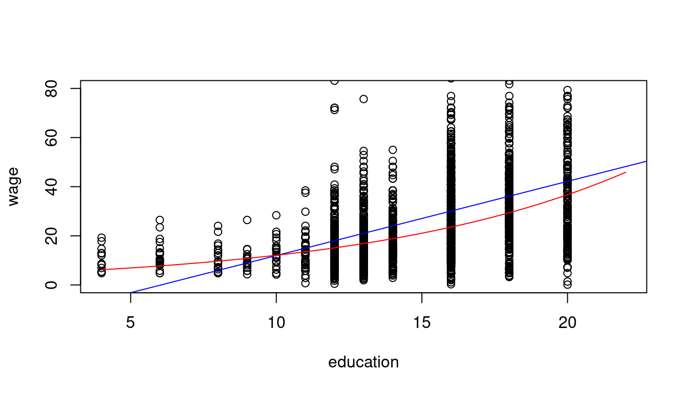
Interpretation: A person with one more year of education has a wage that is 11.13% higher on average.
In addition to the linear-linear and log-linear specifications, we also have the linear-log specification Y = \beta_1 + \beta_2 \log(X) + u and the log-log specification \log(Y) = \beta_1 + \beta_2 \log(X) + u.
Linear-log interpretation: When X is 1\% higher, we observe, on average, a 0.01 \beta_2 higher Y.
Log-log interpretation: When X is 1\% higher, we observe, on average, a \beta_2 \% higher Y.