| person | wage | education | female |
|---|---|---|---|
| 1 | 18.22 | 16 | 1 |
| 2 | 23.85 | 18 | 0 |
| 3 | 10.00 | 16 | 1 |
| 4 | 6.39 | 13 | 0 |
| 5 | 7.42 | 14 | 0 |
1 Data
1.1 Datasets
A univariate dataset is a sequence of observations Y_1, \ldots, Y_n. These n observations can be organized into the data vector \boldsymbol Y, represented as \boldsymbol Y = (Y_1, \ldots, Y_n)'. For example, if you conduct a survey and ask five individuals about their hourly earnings, your data vector might look like \boldsymbol Y = \begin{pmatrix} 18.22 \\ 23.85 \\ 10.00 \\ 6.39 \\ 7.42 \end{pmatrix}. Typically we have data on more than one variable, such as years of education and the gender. Categorical variables are often encoded as dummy variables, which are binary variables. The female dummy variable is defined as 1 if the gender of the person is female and 0 otherwise.
A k-variate dataset is a collection of n vectors \boldsymbol X_1, \ldots, \boldsymbol X_n containing data on k variables. The i-th vector \boldsymbol X_i = (X_{i1}, \ldots, X_{ik})' contains the data on all k variables for individual i. Thus, X_{ij} represents the value for the j-th variable of individual i.
The full k-variate dataset is structured in the n \times k data matrix \boldsymbol X: \boldsymbol X = \begin{pmatrix} \boldsymbol X_1' \\ \vdots \\ \boldsymbol X_n' \end{pmatrix} = \begin{pmatrix} X_{11} & \ldots & X_{1k} \\ \vdots & \ddots & \vdots \\ X_{n1} & \ldots & X_{nk} \end{pmatrix} The i-th row in \boldsymbol X corresponds to the values from \boldsymbol X_i. Since \boldsymbol X_i is a column vector, we use the transpose notation \boldsymbol X_i', which is a row vector. The data matrix and vectors for our example are: \boldsymbol X = \begin{pmatrix} 18.22 & 16 & 1 \\ 23.85 & 18 & 0 \\ 10.00 & 16 & 1 \\ 6.39 & 13 & 0 \\ 7.42 & 14 & 0 \end{pmatrix}, \quad \boldsymbol X_1 = \begin{pmatrix} 18.22 \\ 16 \\ 1 \end{pmatrix}, \boldsymbol X_2 = \begin{pmatrix} 23.85 \\ 18 \\ 0 \end{pmatrix}, \ldots Vector and matrix algebra provide a compact mathematical representation of multivariate data and an efficient framework for analyzing and implementing statistical methods. We will use matrix algebra frequently throughout this course.
To refresh or enhance your knowledge of matrix algebra, please consult the following resources:
Crash Course on Matrix Algebra:
Section 19.1 of the Stock and Watson book also provides a brief overview of matrix algebra concepts.
1.2 R programming language
The best way to learn statistical methods is to program and apply them yourself. Throughout this course, we will use the R programming language for implementing empirical methods and analyzing real-world datasets.
If you are just starting with R, it is crucial to familiarize yourself with its basics. Here’s an introductory tutorial, which contains a lot of valuable resources:
Getting Started with R:
For those new to R, I also recommend the interactive R package SWIRL, which offers an excellent way to learn directly within the R environment. Additionally, two highly recommended online books are Hands-On Programming with R (with focus on programming) and R for Data Science (with focus on data analysis).
One of the best features of R is its extensive ecosystem of packages contributed by the statistical community. You find R packages for almost any statistical method out there and many statisticians provide R packages to accompany their research.
Maybe the most frequently used package is the tidyverse package, which provides a comprehensive suite of data management and visualization tools. You can install the package with the command install.packages("tidyverse") and you can load it with
at the beginning of your code. We will explore several additional packages in the course of the lecture.
1.3 Datasets in R
R includes many built-in datasets and packages of datasets that can be loaded directly into your R environment. For illustration, we consider the penguins dataset available in the palmerpenguins package. To load this dataset into your R session, simply use:
data(penguins, package = "palmerpenguins")
class(penguins)[1] "tbl_df" "tbl" "data.frame"The penguins dataset is stored as a data.frame, R’s most common data storage class for tabular data as in \boldsymbol X. It organizes data in the form of a table, with variables as columns and observations as rows. The penguins object is also identified as a tibble (or tbl_df), the tidyverse version of a data.frame.
To inspect the structure of your dataset, you can use str() or glimpse():
str(penguins)tibble [344 × 8] (S3: tbl_df/tbl/data.frame)
$ species : Factor w/ 3 levels "Adelie","Chinstrap",..: 1 1 1 1 1 1 1 1 1 1 ...
$ island : Factor w/ 3 levels "Biscoe","Dream",..: 3 3 3 3 3 3 3 3 3 3 ...
$ bill_length_mm : num [1:344] 39.1 39.5 40.3 NA 36.7 39.3 38.9 39.2 34.1 42 ...
$ bill_depth_mm : num [1:344] 18.7 17.4 18 NA 19.3 20.6 17.8 19.6 18.1 20.2 ...
$ flipper_length_mm: int [1:344] 181 186 195 NA 193 190 181 195 193 190 ...
$ body_mass_g : int [1:344] 3750 3800 3250 NA 3450 3650 3625 4675 3475 4250 ...
$ sex : Factor w/ 2 levels "female","male": 2 1 1 NA 1 2 1 2 NA NA ...
$ year : int [1:344] 2007 2007 2007 2007 2007 2007 2007 2007 2007 2007 ...The dataset contains variables of various types: fct(factor) for categorical data, dbl(numeric) for real or continuous data, and int(integer) for integer or discrete data. The head() function displays its first few rows:
head(penguins)# A tibble: 6 × 8
species island bill_length_mm bill_depth_mm flipper_length_mm body_mass_g
<fct> <fct> <dbl> <dbl> <int> <int>
1 Adelie Torgersen 39.1 18.7 181 3750
2 Adelie Torgersen 39.5 17.4 186 3800
3 Adelie Torgersen 40.3 18 195 3250
4 Adelie Torgersen NA NA NA NA
5 Adelie Torgersen 36.7 19.3 193 3450
6 Adelie Torgersen 39.3 20.6 190 3650
# ℹ 2 more variables: sex <fct>, year <int>The pipe operator |> efficiently chains commands. It passes the output of one function as the input to another. For example:
  body_mass_g   bill_length_mm       species
 Min.   :2700   Min.   :32.10   Adelie   :152
 1st Qu.:3550   1st Qu.:39.23   Chinstrap: 68
 Median :4050   Median :44.45   Gentoo   :124
 Mean   :4202   Mean   :43.92
 3rd Qu.:4750   3rd Qu.:48.50
 Max.   :6300   Max.   :59.60
 NA's   :2      NA's   :2
The summary() function presents a concise overview, showing absolute frequencies for categorical variables and descriptive statistics for numerical variables, along with information on missing values (NA). To exclude all rows with missing values, we can use na.omit(penguins).
A dummy variable for the penguin species Gentoo can be created with the following command:
gentoo = ifelse(penguins$species == "Gentoo", 1, 0)The $ sign accesses a specific column of a data frame by name, as in penguins$species to select the variable species from penguins.
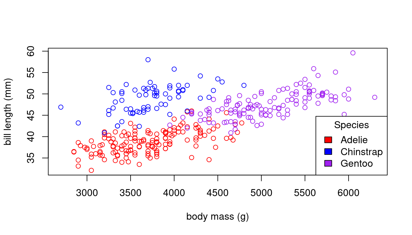
To convert factor variables into dummy variables efficiently, the fastDummies package’s dummy_cols() function can be used. Let’s create dummy variables for each of the three species.
library(fastDummies)
penguins.new = dummy_cols(penguins,select_columns = "species")
Scatterplots provide further insights:
plot(bill_length_mm ~ body_mass_g, data = penguins,
     xlab = "body mass (g)", ylab = "bill length (mm)")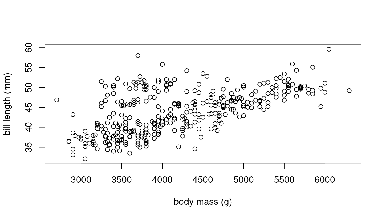
We can assign unique colors to each species:
1.4 Importing data
The internet serves as a vast repository for data in various formats, with csv (comma-separated values), xlsx (Microsoft Excel spreadsheets), and txt (text files) being the most commonly used.
Many organizations, such as the German Bundesbank, the German Federal Statistical Office, the ECB (European Central Bank), Eurostat, and FRED (Federal Reserve Economic Data), offer economic datasets in these formats. These datasets can be accessed through their websites or via Application Programming Interfaces (APIs), which allow direct downloading of data into R. Accessing data via APIs often requires registering for an API token on the organization’s website.
R supports various functions for different data formats:
-
read.csv()for reading comma-separated values -
read.csv2()for semicolon-separated values (adopting the German data convention of using ‘,’ as the decimal mark) -
read.table()for whitespace-separated files -
read_excel()for Microsoft Excel files (requires thereadxlpackage) -
read_stata()for STATA files (requires thehavenpackage)
The rvest package provides web scraping tools to extract data directly from HTML web pages.
In academic writing, it is crucial to provide enough information about data sources to ensure transparency and reproducibility.
Let’s explore the CPS dataset from Bruce Hansen’s website. The Current Population Survey (CPS) is a monthly survey conducted by the U.S. Census Bureau for the Bureau of Labor Statistics, primarily used to measure the labor force status of the U.S. population.
- Dataset: cps09mar.txt
- Description: cps09mar_description.pdf
cps = read.table("https://users.ssc.wisc.edu/~bhansen/econometrics/cps09mar.txt",
        col.names=c("age","female","hisp","education","earnings","hours",
                    "week", "union","uncov","region","race","marital")) |>
  mutate(race = as.factor(race),
         region = as.factor(region),
         marital = as.factor(marital),
         experience = (age - education - 6), #years since graduation
         wage = earnings/(week*hours), #wage per hours
         married = ifelse(marital %in% c(1,2), 1, 0), #dummy
         college = ifelse(education >= 14, 1, 0),
         black = ifelse(race %in% c(2,6,10,11,12,15,16,19), 1, 0),
         asian = ifelse(race %in% c(4,8,11,13,14,16,17,18,19), 1, 0))
1.5 Data types
The most common types of econonomic data are:
Cross-sectional data: Data collected on many entities without regard to time.
Time series data: Data on a single entity collected over multiple time periods.
Panel data: Data collected on multiple entities over multiple time points, combining features of both cross-sectional and time series data.
The cps data is an example of a cross-sectional dataset.
str(cps)Click here to view or hide the output
'data.frame':   50742 obs. of  18 variables:
 $ age       : int  52 38 38 41 42 66 51 49 33 52 ...
 $ female    : int  0 0 0 1 0 1 0 1 0 1 ...
 $ hisp      : int  0 0 0 0 0 0 0 0 0 0 ...
 $ education : int  12 18 14 13 13 13 16 16 16 14 ...
 $ earnings  : int  146000 50000 32000 47000 161525 33000 37000 37000 80000 32000 ...
 $ hours     : int  45 45 40 40 50 40 44 44 40 40 ...
 $ week      : int  52 52 51 52 52 52 52 52 52 52 ...
 $ union     : int  0 0 0 0 1 0 0 0 0 0 ...
 $ uncov     : int  0 0 0 0 0 0 0 0 0 0 ...
 $ region    : Factor w/ 4 levels "1","2","3","4": 1 1 1 1 1 1 1 1 1 1 ...
 $ race      : Factor w/ 20 levels "1","2","3","4",..: 1 1 1 1 1 1 1 1 1 1 ...
 $ marital   : Factor w/ 7 levels "1","2","3","4",..: 1 1 1 1 1 5 1 1 1 1 ...
 $ experience: num  34 14 18 22 23 47 29 27 11 32 ...
 $ wage      : num  62.4 21.4 15.7 22.6 62.1 ...
 $ married   : num  1 1 1 1 1 0 1 1 1 1 ...
 $ college   : num  0 1 1 0 0 0 1 1 1 1 ...
 $ black     : num  0 0 0 0 0 0 0 0 0 0 ...
 $ asian     : num  0 0 0 0 0 0 0 0 0 0 ...
My repository teachingdata contains some recent time series datasets, for instance, the nominal GDP growth of Germany:
Time-Series [1:128] from 1992 to 2024: 0.0874 0.0651 0.0733 0.0586 0.0201 ...The dataset Fatalities is a panel dataset. It contains variables related to traffic fatalities across different states and years in the United States:
Click here to view or hide the output
'data.frame':   336 obs. of  34 variables:
 $ state       : Factor w/ 48 levels "al","az","ar",..: 1 1 1 1 1 1 1 2 2 2 ...
 $ year        : Factor w/ 7 levels "1982","1983",..: 1 2 3 4 5 6 7 1 2 3 ...
 $ spirits     : num  1.37 1.36 1.32 1.28 1.23 ...
 $ unemp       : num  14.4 13.7 11.1 8.9 9.8 ...
 $ income      : num  10544 10733 11109 11333 11662 ...
 $ emppop      : num  50.7 52.1 54.2 55.3 56.5 ...
 $ beertax     : num  1.54 1.79 1.71 1.65 1.61 ...
 $ baptist     : num  30.4 30.3 30.3 30.3 30.3 ...
 $ mormon      : num  0.328 0.343 0.359 0.376 0.393 ...
 $ drinkage    : num  19 19 19 19.7 21 ...
 $ dry         : num  25 23 24 23.6 23.5 ...
 $ youngdrivers: num  0.212 0.211 0.211 0.211 0.213 ...
 $ miles       : num  7234 7836 8263 8727 8953 ...
 $ breath      : Factor w/ 2 levels "no","yes": 1 1 1 1 1 1 1 1 1 1 ...
 $ jail        : Factor w/ 2 levels "no","yes": 1 1 1 1 1 1 1 2 2 2 ...
 $ service     : Factor w/ 2 levels "no","yes": 1 1 1 1 1 1 1 2 2 2 ...
 $ fatal       : int  839 930 932 882 1081 1110 1023 724 675 869 ...
 $ nfatal      : int  146 154 165 146 172 181 139 131 112 149 ...
 $ sfatal      : int  99 98 94 98 119 114 89 76 60 81 ...
 $ fatal1517   : int  53 71 49 66 82 94 66 40 40 51 ...
 $ nfatal1517  : int  9 8 7 9 10 11 8 7 7 8 ...
 $ fatal1820   : int  99 108 103 100 120 127 105 81 83 118 ...
 $ nfatal1820  : int  34 26 25 23 23 31 24 16 19 34 ...
 $ fatal2124   : int  120 124 118 114 119 138 123 96 80 123 ...
 $ nfatal2124  : int  32 35 34 45 29 30 25 36 17 33 ...
 $ afatal      : num  309 342 305 277 361 ...
 $ pop         : num  3942002 3960008 3988992 4021008 4049994 ...
 $ pop1517     : num  209000 202000 197000 195000 204000 ...
 $ pop1820     : num  221553 219125 216724 214349 212000 ...
 $ pop2124     : num  290000 290000 288000 284000 263000 ...
 $ milestot    : num  28516 31032 32961 35091 36259 ...
 $ unempus     : num  9.7 9.6 7.5 7.2 7 ...
 $ emppopus    : num  57.8 57.9 59.5 60.1 60.7 ...
 $ gsp         : num  -0.0221 0.0466 0.0628 0.0275 0.0321 ...
1.6 Random variables
Data is usually the result of a random experiment. The gender of the next person you meet, the daily fluctuation of a stock price, the monthly music streams of your favourite artist, the annual number of pizzas consumed - all of this information involves a certain amount of randomness.
In statistical sciences, we interpret a univariate dataset Y_1, \ldots, Y_n as a sequence of random variables. Similarly, a multivariate dataset \boldsymbol X_1, \ldots, \boldsymbol X_n is viewed as a sequence of random vectors.
Cross-sectional data is typically characterized by an identical distribution across its individual observations, meaning each element in the sequence \boldsymbol X_1, \ldots, \boldsymbol X_n has the same distribution function.
For example, if Y_1, \ldots, Y_n represent the wage levels of different individuals in Germany, each Y_i is drawn from the same distribution F, which in this context is the wage distribution across the country. Similarly, if \boldsymbol X_1, \ldots, \boldsymbol X_n are bivariate random variables containing wages and years of education for individuals, each \boldsymbol X_i follows the same bivariate distribution G, which is the joint distribution of wages and education levels.
A primary goal of econometric methods and statistical inference is to gain insights about features of these true but unknown population distributions F or G using the available data. Econometric methods require certain assumptions about the sampling process and the underlying population distributions. Thus, a solid knowledge of probability theory is essential for econometric modelling.
For a recap on probability theory for econometricians, consider the following refresher:
Probability Theory for Econometricians:
https://probability.svenotto.com/
Section 2 of the Stock and Watson book also provides a review of the most important concepts.
1.7 Sampling
The ideal scenario for data collection involves simple random sampling, where each individual in the population has an equal chance of being selected (independently and identically distributed).
i.i.d. sample
An independently and identically distributed (i.i.d.) sample, or random sample, consists of a sequence of k-variate random vectors \boldsymbol X_1, \ldots, \boldsymbol X_n that have the same probability distribution F and are mutually independent, i.e., for any i \neq j and for all \boldsymbol a, \boldsymbol b \in \mathbb R^k, P(\boldsymbol X_i \leq \boldsymbol a, \boldsymbol X_j \leq \boldsymbol b) = P(\boldsymbol X_i \leq \boldsymbol a) P(\boldsymbol X_j \leq \boldsymbol b).
F is called population distribution or data-generating process (DGP).
The Current Population Survey (CPS) involves random interviews with individuals from the U.S. labor force may be regarded as an i.i.d. sample. Methods like survey sampling, administrative records, direct observation, web scraping, and field/laboratory experiments can yield i.i.d. sampling for economic cross-sectional datasets. In a random sample there is no inherent ordering that would introduce systematic dependencies.
Note that not all cross-sectional data comes from random sampling. For example, clustered sampling occurs when only specific groups (e.g., classrooms) are chosen randomly (students from the same classroom share the same environment and teacher’s performance).
Time series and panel data are intrinsically not independent due to the sequential nature of the observations. We usually expect observations close in time to be strongly dependent and observations at greater distances to be less dependent.
For time series data we assume that there exists some underlying stochastic process represented as a doubly infinite sequence of random variables \{ Y_t \}_{t \in \mathbb Z} = \{ \ldots, Y_{-1}, Y_0, \underbrace{Y_1, \ldots, Y_n}_{\text{observed part}}, Y_{n+1}, \ldots \}, where the time series sample \{Y_1, \ldots, Y_n\} is only the observed part of the process.
In order to learn from the observed part about the future (forecasting) or make inference on the dependence with other variables, we typically assume that the distribution of the time series sample does not depend on which time periods are observed, which excludes structural breaks or stochastic trends.
Stationary time series
A time series process \{Y_i\}_{i \in \mathbb Z} is called stationary if the mean \mu and the autocovariances \gamma(\tau) do not depend on the time point i. That is, \mu := E[Y_i] < \infty, \quad \text{for all} \ i, and \gamma(\tau) := Cov(Y_i, Y_{i-\tau}) < \infty \quad \text{for all} \ i \ \text{and} \ \tau.
The quarterly nominal GDP is clearly nonstationary. It exhibits trending behavior and seasonalities. The annual nominal GDP growth rates can be regarded as a stationary time series.
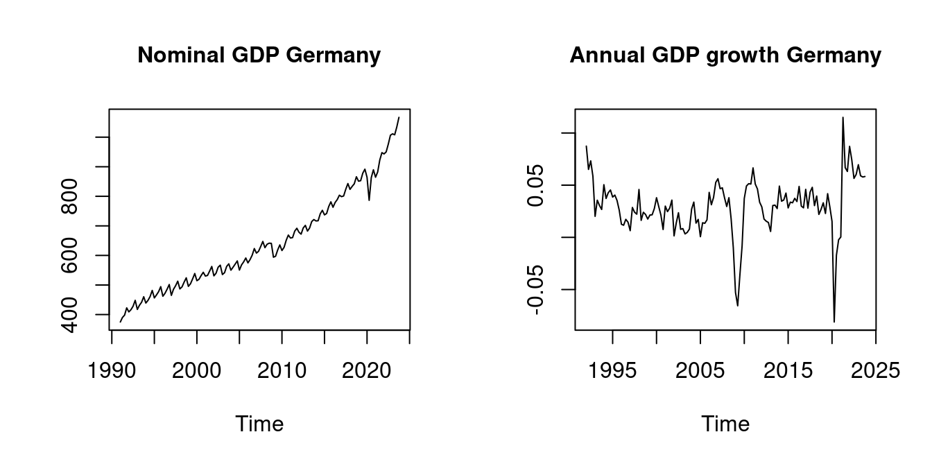
Macroeconomic time series often indicate trending behavior and/or seasonalities. However, we can often use simple transformations to convert nonstationary time series into stationary series, such as differences (diff(your_series, your_frequency)) or growth rates (diff(log(your_series), your_frequency)).
The frequency is the number of observed periods per time basis. Time series (ts) objects in R are defined in terms of a yearly time basis. Yearly time series have frequency 1, quarterly have frequency 4, and monthly have frequency 12.
Here are some common transformations:
- First differences: \Delta Y_i = Y_i - Y_{i-1}
- Growth rates: \log(Y_i) - \log(Y_{i-1})
For seasonal data with frequency 4:
- Fourth differences: \Delta Y_i = Y_i - Y_{i-4}
- Annual growth rates: \log(Y_i) - \log(Y_{i-4})