2  Summary Statistics

PDF version

In this section you find an overview of the most important summary statistics commands. In the table below, your_data represents some univariate data (vector), and your_df represents a data.frame of multivariate data (matrix).

Statistic	Command
Sample Size (n)	length(your_data)
Maximum Value	max(your_data)
Minimum Value	min(your_data)
Total Sum	sum(your_data)
Mean	mean(your_data)
Variance	var(your_data)
Standard Deviation	sd(your_data)
Skewness	skewness(your_data) (requires moments package)
Kurtosis	kurtosis(your_data) (requires moments package)
Order statistics	sort(your_data)
Empirical CDF	ecdf(your_data)
Median	median(your_data)
p-Quantile	quantile(your_data, p)
Boxplot	boxplot(your_data)
Histogram	hist(your_data)
Kernel density estimator	plot(density(your_data))
Covariance	cov(your_data1, your_data2)
Correlation	cor(your_data1, your_data2)
Mean vector	colMeans(your_df)
Covariance matrix	cov(your_df)
Correlation matrix	cor(your_df)

Note: Ensure that your data does not contain missing values (NA’s) for these commands. Use na.omit() or include na.rm=TRUE in functions to handle missing data.

2.1 Sample moments

Mean

The sample mean (arithmetic mean) is the most common measure of central tendency: $$\overline Y = \frac{1}{n} \sum_{i=1}^n Y_i$$ In i.i.d. samples, it converges in probability to the expected value as sample size grows (law of large numbers). I.e., it is a consistent estimator for the population mean: $$\overline Y \overset{p}{\rightarrow} E[Y] \quad \text{as} \ n \to \infty.$$ The law of large numbers also holds for stationary time series with $\gamma(\tau) \to 0$ as $\tau \to \infty$.

Variance

The variance measures the spread around the mean. The sample variance is $$\widehat \sigma_Y^2 = \frac{1}{n} \sum_{i=1}^n (Y_i - \overline Y)^2 = \overline{Y^2} - \overline Y^2,$$ and the adjusted sample variance is $$s_Y^2 = \frac{1}{n-1} \sum_{i=1}^n (Y_i - \overline Y)^2.$$ Note that var(your_data) computes $s^2_Y$, which is the conventional estimator for the population variance $$Var[Y] = E[(Y - E[Y])^2] = E[Y^2] - E[Y]^2.$$ $s_Y^2$ is unbiased whereas $\widehat \sigma_Y^2$ is biased but has a lower sampling variance. For i.i.d. samples, both versions are consistent estimators for the population variance.

Standard deviation

The standard deviation, the square root of the variance, is a measure of dispersion in the original unit of data. It quantifies the average distance data points typically deviate from the mean of their distribution.

The sample standard deviation and its adjusted version are the square roots of the corresponding variance formulas: $$\widehat \sigma_Y = \sqrt{\overline{Y^2} - \overline Y^2}, \quad s_Y = \sqrt{\frac{1}{n-1} \sum_{i=1}^n (Y_i - \overline Y)^2}$$ Note that sd(your_data) computes $s_Y$ and not $\widehat \sigma_Y$. Both versions are consistent estimators for the population standard deviation $sd(Y) = \sqrt{Var[Y]}$ for i.i.d. samples.

Skewness

The skewness is a measure of asymmetry around the mean. The sample skewness is $$\widehat{skew} = \frac{1}{n \widehat \sigma_Y^3} \sum_{i=1}^n (Y_i - \overline Y)^3.$$ It is a consistent estimator for the population skewness $$skew = \frac{E[(Y - E[Y])^3]}{sd(Y)^3}.$$ A non-zero skewness indicates an asymmetric distribution, with positive values indicating a right tail and negative values a left tail. Below you find an illustration using density functions:

Figure 2.1

Kurtosis

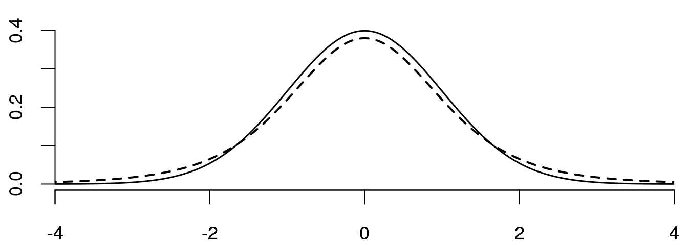
Kurtosis measures the heaviness of the tails of a distribution. It indicates how likely extreme outliers are. The sample kurtosis is $$\widehat{kurt} = \frac{1}{n \widehat \sigma_Y^4} \sum_{i=1}^n (Y_i - \overline Y)^4.$$ It is a consistent estimator for the population kurtosis $$kurt = \frac{E[(Y - E[Y])^4]}{Var[Y]^2}.$$ The reference value is 3, which is the kurtosis of the standard normal distribution $\mathcal N(0,1)$.

Values significantly above 3 indicate a distribution with heavy tails, such as the t-distribution $t(5)$ with a kurtosis of 9, implying a higher likelihood of outliers compared to $\mathcal{N}(0,1)$. Conversely, a distribution with kurtosis significantly below 3, such as the uniform distribution (kurt = 1.8), is called light-tailed, indicating fewer outliers. Both skewness and kurtosis are unit free measures.

Below you find the probability densities of the $\mathcal N(0,1)$ (solid) and the $t(5)$ (dashed) distributions:

Higher Moments

The $r$-th sample moment is $$\overline{Y^r} = \frac{1}{n} \sum_{i=1}^n Y_i^r.$$ The sample mean is the first sample moment. The variance is the second minus the first squared sample moment (centered sample moment). The standard deviation, skewness, and kurtosis are also functions of the first four sample moments.

library(moments)
data(penguins, package="palmerpenguins")
Y = na.omit(penguins$body_mass_g)
length(Y)
max(Y)
min(Y)
sum(Y)
mean(Y)
var(Y)
sd(Y)
skewness(Y)
kurtosis(Y)

2.2 Empirical distribution

The distribution $F$ of a random variable $Y$ is defined by its cumulative distribution function (CDF) $$F(a) = P(Y \leq a), \quad a \in \mathbb R.$$ With knowledge of $F(\cdot)$, you can calculate the probability of $Y$ falling within any interval $I \subseteq \mathbb{R}$, or any countable union of such intervals, by applying the rules of probability.

The empirical cumulative distribution function (ECDF) is the sample-based counterpart of the CDF. It represents the proportion of observations within the sample that are less than or equal to a certain value $a$. To define the ECDF in mathematical terms, we use the concept of order statistics $Y_{(h)}$, which is the sample data arranged in ascending order such that $$Y_{(1)} \leq Y_{(2)} \leq \ldots \leq Y_{(n)}.$$ You can obtain the order statistics for your dataset using sort(your_data).

The ECDF is then defined as $$\widehat F(a) = \begin{cases} 0 & \text{for} \ a \in \big(-\infty, Y_{(1)}\big), \\ \frac{k}{n} & \text{for} \ a \in \big[Y_{(k)}, Y_{(k+1)}\big), \\ 1 & \text{for} \ a \in \big[Y_{(n)}, \infty \big). \end{cases}$$ The ECDF is always a step function with steps becoming arbitrarily small for continuous distributions as $n$ increases. The ECDF is a consistent estimator for the CDF if the sample is i.i.d. (Glivenko–Cantelli theorem): $$\sup_{a \in \mathbb R} |\widehat F(a) - F(a)| \overset{p}{\rightarrow} 0 \quad \text{as} \ n \to \infty.$$

data(penguins, package="palmerpenguins")
plot(ecdf(penguins$bill_length_mm))

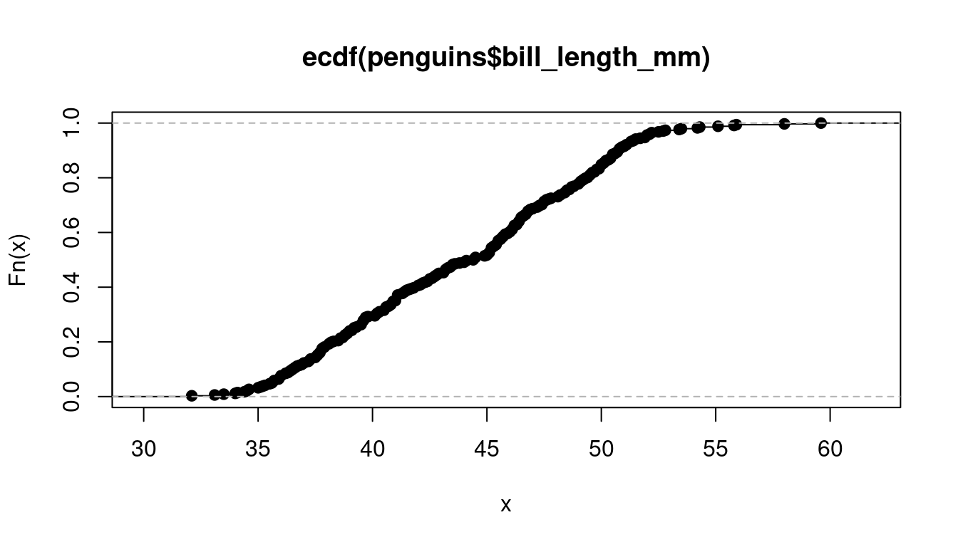
Have a look at the ECDF’s of the variables wage, education, and female from the cps data.

2.3 Sample quantiles

Median

The median is a central value that splits the distribution into two equal parts.

For a continuous distribution, the population median is the value $med$ such that $F(med) = 0.5$. In discrete distributions, if $F$ is flat where it takes the value 0.5, the median isn’t uniquely defined as any value within this flat region could technically satisfy the median condition $F(med) = 0.5$.

The empirical median of a sorted dataset is found at the point where the ECDF reaches 0.5. For an even-sized dataset, the median is the average of the two central observations:

$$\widehat{med} = \begin{cases} Y_{(\frac{n+1}{2})} & \text{if} \ n \ \text{is odd} \\ \frac{1}{2} \big( Y_{(\frac{n}{2})} + Y_{(\frac{n}{2}+1)} \big) & \text{if} \ n \ \text{is even} \end{cases}$$ The median corresponds to the 0.5-quantile of the distribution.

Quantile

The population $p$-quantile is the value $q_p$ such that $F(q_p) = p$. Similarly to the population median, population quantiles may not be unique for discrete distributions.

The emirical $p$-quantile $\widehat q_p$ is a value at which $p$ percent of the data falls below it. It can be computed as the linear interpolation at $h=(n-1)p+1$ between $Y_{(\lfloor h \rfloor)}$ and $Y_{(\lceil h \rceil)}$: $$\widehat{q}_p = Y_{(\lfloor h \rfloor)} + (h - \lfloor h \rfloor) (Y_{(\lceil h \rceil)} - Y_{(\lfloor h \rfloor)}).$$ This interpolation scheme is standard in R, although multiple approaches exist for estimating quantiles (see here).

Boxplot

Boxplots graphically represent the empirical distribution.

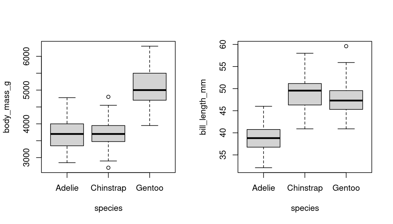
The box indicates the interquartile range ($IQR = \widehat q_{0.75} - \widehat q_{0.25}$) and the median of the dataset. The upper whisker indicates the largest observation that does not exceed $\widehat q_{0.75} + 1.5 IQR$, and the lower whisker is the smallest observation that is greater or equal to $\widehat q_{0.25} - 1.5 IQR$. The points beyond the $1.5 IQR$ distance are plotted as single points and indicate potential outliers or the presence of a skewed or heavy tailed distribution.

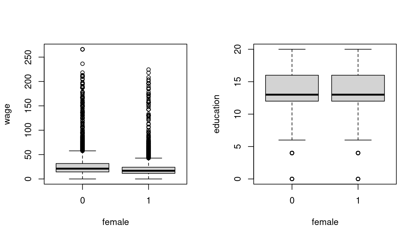
Boxplots are helpful for comparing distributions across groups, such as differences in body mass or bill length among penguin species, or wage distributions by gender:

par(mfrow = c(1,2), cex=0.9)
boxplot(body_mass_g ~ species, data = penguins)
boxplot(bill_length_mm ~ species, data = penguins)

boxplot(wage ~ female, data = cps)
boxplot(education ~ female, data = cps)

2.4 Density estimation

A continuous random variable $Y$ is characterized by a continuously differentiable CDF $F(a) = P(Y \leq a)$. The derivative is known as the probability density function (PDF), defined as $f(a) = F'(a)$. A simple method to estimate $f$ is through the construction of a histogram.

Histogram

A histogram divides the data range into $B$ bins each of equal width $h$ and counts the number of observations $n_j$ within each bin. The histogram estimator of $f(a)$ for $a$ in the $j$-th bin is $$\widehat f(a) = \frac{n_j}{nh}.$$ The histogram is the plot of these heights, displayed as rectangles, with their area normalized so that the total area equals 1. The appearance and accuracy of a histogram depend on the choice of bin width $h$.

Let’s consider the subset of the CPS dataset of Asian women, excluding those with wages over $80 for illustrative purposes:

library(tidyverse)
cps.new = cps |> filter(asian == 1, female == 1, wage < 80)
wage = cps.new$wage
par(mfrow = c(1,3))
hist(wage, breaks = seq(0,80,by=20), probability = TRUE, main = "h=20")
hist(wage, breaks = seq(0,80,by=10), probability = TRUE, main = "h=10")
hist(wage, breaks = seq(0,80,by=1), probability = TRUE, main = "h=1")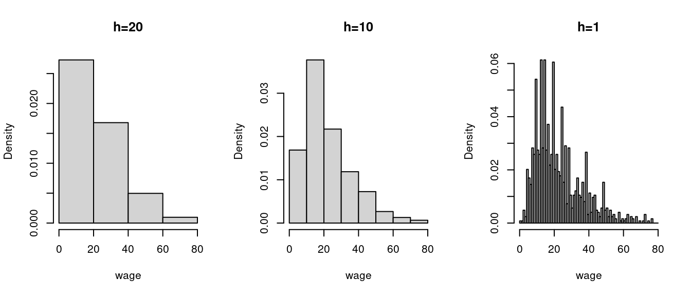

Running hist(wage, probability=TRUE) automatically selects a suitable bin width. hist(wage)$breaks shows the automatically selected break poins, where the bin width is the distance between break points.

Kernel density estimator

Suppose we want to estimate the wage density at $a = 22$ and consider the histogram density estimate in the figure above with $h=10$. It is based on the frequency of observations in the interval $[20, 30)$ which is a skewed window about $a = 22$.

It seems more sensible to center the window at 22, for example $[17, 27)$ instead of $[20, 30)$. It also seems sensible to give more weight to observations close to 22 and less to those at the edge of the window.

This idea leads to the kernel density estimator of $f(a)$, which is a smooth version of the histogram:

$$\widehat f(a) = \frac{1}{nh} \sum_{i=1}^n K\Big(\frac{X_i - a}{h} \Big).$$ Here, $K(u)$ represents a weighting function known as a kernel function, and $h > 0$ is the bandwidth. A common choice for $K(u)$ is the Gaussian kernel: $$K(u) = \phi(u) = \frac{1}{\sqrt{2 \pi}} \exp(-u^2/2).$$

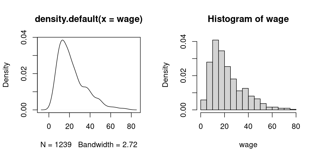
The density() function in R automatically selects an optimal bandwidth, but it also allows for manual bandwidth specification via density(wage, bw = your_bandwidth).

2.5 Sample covariance

Consider a multivariate dataset $\boldsymbol X_1, \ldots, \boldsymbol X_n$ represented as an $n \times k$ data matrix $\boldsymbol X = (\boldsymbol X_1, \ldots, \boldsymbol X_n)'$. For example, the following subset of the penguins dataset:

peng = penguins |> 
  select(bill_length_mm, flipper_length_mm, body_mass_g) |> 
  na.omit()

Sample mean vector

The sample mean vector $\overline{\boldsymbol X}$ is defined as $$\overline{\boldsymbol X} = \frac{1}{n} \sum_{i=1}^n \boldsymbol X_i.$$ It is a consistent estimator for the population mean vector $E[\boldsymbol X_i]$ if the sample is i.i.d..

colMeans(peng)

   bill_length_mm flipper_length_mm       body_mass_g 
         43.92193         200.91520        4201.75439 

Sample covariance matrix

The adjusted sample covariance matrix $\widehat{\boldsymbol \Sigma}$ is defined as the $k \times k$ matrix $$\widehat{\boldsymbol \Sigma} = \frac{1}{n-1} \sum_{i=1}^n (\boldsymbol X_i - \overline{\boldsymbol X})(\boldsymbol X_i - \overline{\boldsymbol X})',$$ where its $(h,l)$ element is the pairwise sample covariance of variable $h$ and $l$ given by $$s_{h,l} = \frac{1}{n-1} \sum_{i=1}^n (X_{ih} -\overline{\boldsymbol X}_h)(X_{il} - \overline{\boldsymbol X}_l), \quad \overline{\boldsymbol X}_h = \frac{1}{n} \sum_{i=1}^n X_{ih}.$$

If the sample is i.i.d., $\widehat{\boldsymbol \Sigma}$ is an unbiased and consistent estimator for the population covariance matrix $E[(\boldsymbol X_i - E[\boldsymbol X_i])(\boldsymbol X_i - E[\boldsymbol X_i])']$.

cov(peng)

                  bill_length_mm flipper_length_mm body_mass_g
bill_length_mm          29.80705          50.37577    2605.592
flipper_length_mm       50.37577         197.73179    9824.416
body_mass_g           2605.59191        9824.41606  643131.077

Sample correlation matrix

The correlation matrix is the matrix containing the pairwise sample correlation coefficients $$r_{h,l} = \frac{\sum_{i=1}^n (X_{ih} -\overline{\boldsymbol X}_h)(X_{il} - \overline{\boldsymbol X}_l)}{\sqrt{\sum_{i=1}^n (X_{ih} -\overline{\boldsymbol X}_h)^2}\sqrt{\sum_{i=1}^n (X_{il} -\overline{\boldsymbol X}_l)^2}}.$$

cor(peng)

                  bill_length_mm flipper_length_mm body_mass_g
bill_length_mm         1.0000000         0.6561813   0.5951098
flipper_length_mm      0.6561813         1.0000000   0.8712018
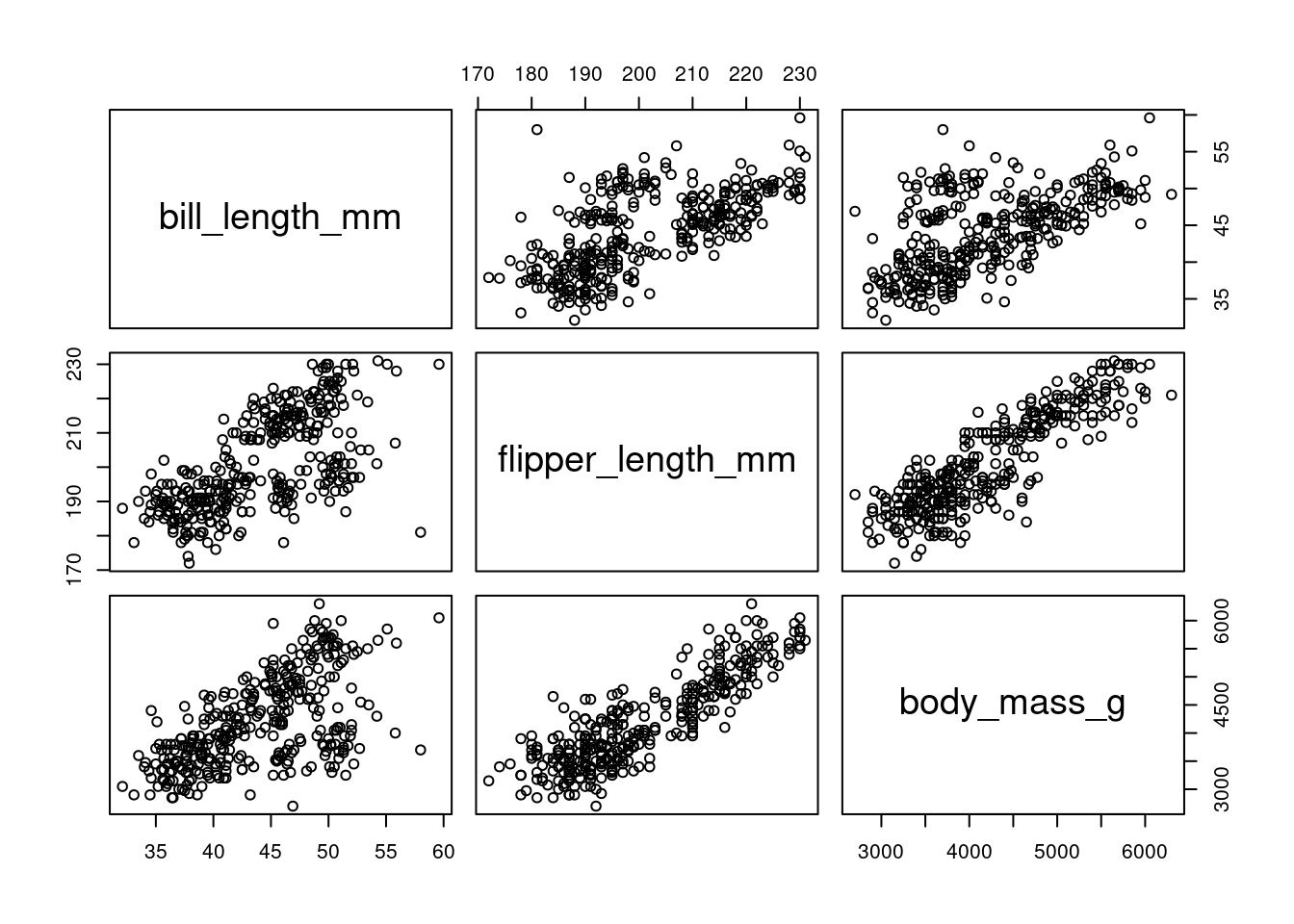
body_mass_g            0.5951098         0.8712018   1.0000000

Both the covariance and correlation matrices are symmetric The scatterplots of the full dataset visualize the positive correlations between the variables in the penguins data:

plot(peng)

2.6 R-codes

methods-sec02.R