library(dynlm)  # for dynamic linear models
data(gdpgr, package = "teachingdata")
plot(gdpgr, main = "Nominal monthly GDP growth Germany")
Consider two time series Y_t and Z_t for t=1, \ldots, T. The index t is used instead of i because observations correspond to time points, not individuals. T represents the sample size, i.e., the number of observed time periods.
Here are some core linear time series forecasting models:
In these equations, p is the number of lags of the dependent variable Y_t, q is the number of lags of the explanatory variable Z_t, and u_t is a mean zero error (shock) that is conditional mean independent of the regressors. These models can be estimated by OLS.
The AR, DL, and ADL models can be used for forecasting because the regressors lie in the past relative to the dependent variable. Further exogenous variables can also be included.
If the model parameters are known and the sample is given for t=1, \ldots, T, we can compute the out-of-sample predicted value for t=T+1, which defines a population forecast for Y_{T+1} (1-step ahead forecast). E.g. in the ADL model, we have Y_{T+1|T} = \alpha_0 + \alpha_1 Y_{T} + \ldots + \alpha_p Y_{T-p+1} + \delta_1 Z_{T} + \ldots + \delta_q Z_{T-q+1}. Using estimated coefficients, we have the 1-step ahead forecast \widehat Y_{T+1|T} = \widehat \alpha_0 + \widehat \alpha_1 Y_{T} + \ldots + \widehat \alpha_p Y_{T-p+1} + \widehat \delta_1 Z_{T} + \ldots + \widehat \delta_q Z_{T-q+1}.
Because regression models with time series variables typically include lags of variables, we call them dynamic regression models.
In general, let Y_t be the univariate dependent time series variable, and \boldsymbol X_t = (X_{1t}, \ldots, X_{kt})' be the k-variate regressor time series vector. A time series regression is a linear regression model Y_t = \boldsymbol X_t' \boldsymbol \beta + u_t, \quad t=1, \ldots, T, \qquad \quad \tag{14.1} where the error term satisfies E[u_t|\boldsymbol X_t] = 0.
The vector of regressors \boldsymbol X_t may contain multiple exogenous variables and its lags, but also lags of the dependent variable. E.g., in the ADL(p,q) model, we have k=p+q+1 and \begin{align*} \boldsymbol X_t &= (1, Y_{t-1} ,\ldots, Y_{t-p}, Z_{t-1}, \ldots, Z_{t-q})', \\ \boldsymbol \beta &= (\alpha_0, \alpha_1, \ldots, \alpha_p, \delta_1, \ldots, \delta_q)'. \end{align*}
The OLS estimator is \widehat{\boldsymbol \beta} = \bigg( \sum_{t=1}^T \boldsymbol X_t \boldsymbol X_t' \bigg)^{-1} \bigg( \sum_{t=1}^T \boldsymbol X_t Y_t \bigg).
To compute \boldsymbol X_1 in \widehat{\boldsymbol \beta} for dynamic models, we need a few additional observations at the beginning of the sample. I.e., for the ADL(p,q) model, Y_t must be observed from t=1-p, \ldots, T and Z_t from t=1-q, \ldots, T.
In forecasting models, the regressors contain only variables that lie in the past of t. Therefore, \boldsymbol X_{T+1} is known from the sample, and the one-step ahead forecast can be computed as \widehat Y_{T+1|T} = \boldsymbol X_{T+1}'\widehat{\boldsymbol \beta}. The forecast error is \begin{align*} f_{T+1|T} &= Y_{T+1} - \widehat Y_{T+1|T} \\ &= \boldsymbol X_{T+1}'\boldsymbol \beta + u_{T+1} - \boldsymbol X_{T+1}'\widehat{\boldsymbol \beta} \\ &= u_{T+1} + \boldsymbol X_{T+1}'(\boldsymbol \beta - \widehat{\boldsymbol \beta}) \\ &\approx u_{T+1}. \end{align*} The last step holds for large T if the OLS estimator \widehat{\boldsymbol \beta} is consistent.
To obtain a (1-\alpha)-forecast interval I_{(T+1|T; 1-\alpha)} with \lim_{T\to \infty} P\Big(Y_{T+1} \in I_{(T+1|T; 1-\alpha)}\Big) = 1-\alpha, \qquad \quad \tag{14.2} we require a distributional assumption for the error term. Unfortunately, the central limit theorem will not help us here. The most common assumption is to assume normally distributed errors u_t \sim \mathcal N(0, \sigma^2), but also a t-distribution is possible if there is evidence that the errors have a higher kurtosis.
If the errors are normally distributed and the OLS estimator is consistent, it follows that \lim_{T \to \infty} P\bigg(\frac{f_{T+1|T}}{s_{\widehat u}} \leq c\bigg) = \Phi(c), where \Phi is the standard normal CDF. Consequently, Equation 14.2 holds with I_{(T+1|T;1-\alpha)} = \Big[\widehat Y_{T+1|T} - z_{(1-\frac{\alpha}{2})} s_{\widehat u}; \widehat Y_{T+1|T} + z_{(1-\frac{\alpha}{2})} s_{\widehat u} \Big], where s_{\widehat u} is the standard error of regression (SER).
library(dynlm) # for dynamic linear models
data(gdpgr, package = "teachingdata")
plot(gdpgr, main = "Nominal monthly GDP growth Germany")
Consider the AR(4) model for GDP growth: gdp_t = \alpha_0 + \alpha_1 gdp_{t-1} + \alpha_2 gdp_{t-2} + \alpha_3 gdp_{t-3} + \alpha_4 gdp_{t-4} + u_t.
One challenge is to define the lagged regressors correctly. Because we have four lags, we need T+4 observations from t=-3, \ldots, T to compute the OLS estimate. The embed() function is useful to get the regressor matrix with the shifted variables with lags from 1 to 4:
embed(gdpgr,5) [,1] [,2] [,3] [,4] [,5]
[1,] 0.0201337715 0.0586045514 0.0732642826 0.0651053628 0.0874092348
[2,] 0.0355929601 0.0201337715 0.0586045514 0.0732642826 0.0651053628
[3,] 0.0305325110 0.0355929601 0.0201337715 0.0586045514 0.0732642826
[4,] 0.0267275508 0.0305325110 0.0355929601 0.0201337715 0.0586045514
[5,] 0.0504532397 0.0267275508 0.0305325110 0.0355929601 0.0201337715
[6,] 0.0372759162 0.0504532397 0.0267275508 0.0305325110 0.0355929601
[7,] 0.0427747084 0.0372759162 0.0504532397 0.0267275508 0.0305325110
[8,] 0.0453798176 0.0427747084 0.0372759162 0.0504532397 0.0267275508
[9,] 0.0385844643 0.0453798176 0.0427747084 0.0372759162 0.0504532397
[10,] 0.0404915385 0.0385844643 0.0453798176 0.0427747084 0.0372759162
[11,] 0.0353187251 0.0404915385 0.0385844643 0.0453798176 0.0427747084
[12,] 0.0260446862 0.0353187251 0.0404915385 0.0385844643 0.0453798176
[13,] 0.0125448113 0.0260446862 0.0353187251 0.0404915385 0.0385844643
[14,] 0.0116162653 0.0125448113 0.0260446862 0.0353187251 0.0404915385
[15,] 0.0172743837 0.0116162653 0.0125448113 0.0260446862 0.0353187251
[16,] 0.0145381167 0.0172743837 0.0116162653 0.0125448113 0.0260446862
[17,] 0.0064074433 0.0145381167 0.0172743837 0.0116162653 0.0125448113
[18,] 0.0286181410 0.0064074433 0.0145381167 0.0172743837 0.0116162653
[19,] 0.0240593231 0.0286181410 0.0064074433 0.0145381167 0.0172743837
[20,] 0.0222180983 0.0240593231 0.0286181410 0.0064074433 0.0145381167
[21,] 0.0458560754 0.0222180983 0.0240593231 0.0286181410 0.0064074433
[22,] 0.0162997134 0.0458560754 0.0222180983 0.0240593231 0.0286181410
[23,] 0.0240238678 0.0162997134 0.0458560754 0.0222180983 0.0240593231
[24,] 0.0219259244 0.0240238678 0.0162997134 0.0458560754 0.0222180983
[25,] 0.0175312705 0.0219259244 0.0240238678 0.0162997134 0.0458560754
[26,] 0.0213872237 0.0175312705 0.0219259244 0.0240238678 0.0162997134
[27,] 0.0215996987 0.0213872237 0.0175312705 0.0219259244 0.0240238678
[28,] 0.0275603181 0.0215996987 0.0213872237 0.0175312705 0.0219259244
[29,] 0.0379630756 0.0275603181 0.0215996987 0.0213872237 0.0175312705
[30,] 0.0295828692 0.0379630756 0.0275603181 0.0215996987 0.0213872237
[31,] 0.0213309511 0.0295828692 0.0379630756 0.0275603181 0.0215996987
[32,] 0.0075237667 0.0213309511 0.0295828692 0.0379630756 0.0275603181
[33,] 0.0299392612 0.0075237667 0.0213309511 0.0295828692 0.0379630756
[34,] 0.0246649062 0.0299392612 0.0075237667 0.0213309511 0.0295828692
[35,] 0.0280194737 0.0246649062 0.0299392612 0.0075237667 0.0213309511
[36,] 0.0356734942 0.0280194737 0.0246649062 0.0299392612 0.0075237667
[37,] 0.0014322600 0.0356734942 0.0280194737 0.0246649062 0.0299392612
[38,] 0.0138416969 0.0014322600 0.0356734942 0.0280194737 0.0246649062
[39,] 0.0235678950 0.0138416969 0.0014322600 0.0356734942 0.0280194737
[40,] 0.0077007205 0.0235678950 0.0138416969 0.0014322600 0.0356734942
[41,] 0.0083826875 0.0077007205 0.0235678950 0.0138416969 0.0014322600
[42,] 0.0032922145 0.0083826875 0.0077007205 0.0235678950 0.0138416969
[43,] 0.0047364761 0.0032922145 0.0083826875 0.0077007205 0.0235678950
[44,] 0.0079743278 0.0047364761 0.0032922145 0.0083826875 0.0077007205
[45,] 0.0270819565 0.0079743278 0.0047364761 0.0032922145 0.0083826875
[46,] 0.0337685936 0.0270819565 0.0079743278 0.0047364761 0.0032922145
[47,] 0.0136382992 0.0337685936 0.0270819565 0.0079743278 0.0047364761
[48,] 0.0172059191 0.0136382992 0.0337685936 0.0270819565 0.0079743278
[49,] 0.0006541173 0.0172059191 0.0136382992 0.0337685936 0.0270819565
[50,] 0.0139693816 0.0006541173 0.0172059191 0.0136382992 0.0337685936
[51,] 0.0134547959 0.0139693816 0.0006541173 0.0172059191 0.0136382992
[52,] 0.0167457829 0.0134547959 0.0139693816 0.0006541173 0.0172059191
[53,] 0.0430703460 0.0167457829 0.0134547959 0.0139693816 0.0006541173
[54,] 0.0312473976 0.0430703460 0.0167457829 0.0134547959 0.0139693816
[55,] 0.0382467143 0.0312473976 0.0430703460 0.0167457829 0.0134547959
[56,] 0.0526367957 0.0382467143 0.0312473976 0.0430703460 0.0167457829
[57,] 0.0561884737 0.0526367957 0.0382467143 0.0312473976 0.0430703460
[58,] 0.0466371217 0.0561884737 0.0526367957 0.0382467143 0.0312473976
[59,] 0.0474469210 0.0466371217 0.0561884737 0.0526367957 0.0382467143
[60,] 0.0378900574 0.0474469210 0.0466371217 0.0561884737 0.0526367957
[61,] 0.0295752497 0.0378900574 0.0474469210 0.0466371217 0.0561884737
[62,] 0.0379954321 0.0295752497 0.0378900574 0.0474469210 0.0466371217
[63,] 0.0178515785 0.0379954321 0.0295752497 0.0378900574 0.0474469210
[64,] -0.0099977546 0.0178515785 0.0379954321 0.0295752497 0.0378900574
[65,] -0.0528038611 -0.0099977546 0.0178515785 0.0379954321 0.0295752497
[66,] -0.0655685839 -0.0528038611 -0.0099977546 0.0178515785 0.0379954321
[67,] -0.0361084433 -0.0655685839 -0.0528038611 -0.0099977546 0.0178515785
[68,] -0.0083350789 -0.0361084433 -0.0655685839 -0.0528038611 -0.0099977546
[69,] 0.0372744742 -0.0083350789 -0.0361084433 -0.0655685839 -0.0528038611
[70,] 0.0492404647 0.0372744742 -0.0083350789 -0.0361084433 -0.0655685839
[71,] 0.0514080371 0.0492404647 0.0372744742 -0.0083350789 -0.0361084433
[72,] 0.0510942532 0.0514080371 0.0492404647 0.0372744742 -0.0083350789
[73,] 0.0665344115 0.0510942532 0.0514080371 0.0492404647 0.0372744742
[74,] 0.0511323253 0.0665344115 0.0510942532 0.0514080371 0.0492404647
[75,] 0.0463615981 0.0511323253 0.0665344115 0.0510942532 0.0514080371
[76,] 0.0336752941 0.0463615981 0.0511323253 0.0665344115 0.0510942532
[77,] 0.0291605087 0.0336752941 0.0463615981 0.0511323253 0.0665344115
[78,] 0.0175460213 0.0291605087 0.0336752941 0.0463615981 0.0511323253
[79,] 0.0154886280 0.0175460213 0.0291605087 0.0336752941 0.0463615981
[80,] 0.0142225002 0.0154886280 0.0175460213 0.0291605087 0.0336752941
[81,] 0.0056581603 0.0142225002 0.0154886280 0.0175460213 0.0291605087
[82,] 0.0305069664 0.0056581603 0.0142225002 0.0154886280 0.0175460213
[83,] 0.0308774823 0.0305069664 0.0056581603 0.0142225002 0.0154886280
[84,] 0.0276026912 0.0308774823 0.0305069664 0.0056581603 0.0142225002
[85,] 0.0490999652 0.0276026912 0.0308774823 0.0305069664 0.0056581603
[86,] 0.0346488227 0.0490999652 0.0276026912 0.0308774823 0.0305069664
[87,] 0.0358017884 0.0346488227 0.0490999652 0.0276026912 0.0308774823
[88,] 0.0424204059 0.0358017884 0.0346488227 0.0490999652 0.0276026912
[89,] 0.0282154475 0.0424204059 0.0358017884 0.0346488227 0.0490999652
[90,] 0.0337444820 0.0282154475 0.0424204059 0.0358017884 0.0346488227
[91,] 0.0331285814 0.0337444820 0.0282154475 0.0424204059 0.0358017884
[92,] 0.0373844847 0.0331285814 0.0337444820 0.0282154475 0.0424204059
[93,] 0.0343197078 0.0373844847 0.0331285814 0.0337444820 0.0282154475
[94,] 0.0487914477 0.0343197078 0.0373844847 0.0331285814 0.0337444820
[95,] 0.0299897045 0.0487914477 0.0343197078 0.0373844847 0.0331285814
[96,] 0.0282785948 0.0299897045 0.0487914477 0.0343197078 0.0373844847
[97,] 0.0459681771 0.0282785948 0.0299897045 0.0487914477 0.0343197078
[98,] 0.0279843861 0.0459681771 0.0282785948 0.0299897045 0.0487914477
[99,] 0.0433567397 0.0279843861 0.0459681771 0.0282785948 0.0299897045
[100,] 0.0479289263 0.0433567397 0.0279843861 0.0459681771 0.0282785948
[101,] 0.0304271605 0.0479289263 0.0433567397 0.0279843861 0.0459681771
[102,] 0.0395955660 0.0304271605 0.0479289263 0.0433567397 0.0279843861
[103,] 0.0219910435 0.0395955660 0.0304271605 0.0479289263 0.0433567397
[104,] 0.0268311490 0.0219910435 0.0395955660 0.0304271605 0.0479289263
[105,] 0.0330945264 0.0268311490 0.0219910435 0.0395955660 0.0304271605
[106,] 0.0228782682 0.0330945264 0.0268311490 0.0219910435 0.0395955660
[107,] 0.0418425360 0.0228782682 0.0330945264 0.0268311490 0.0219910435
[108,] 0.0292072118 0.0418425360 0.0228782682 0.0330945264 0.0268311490
[109,] 0.0152491384 0.0292072118 0.0418425360 0.0228782682 0.0330945264
[110,] -0.0811063878 0.0152491384 0.0292072118 0.0418425360 0.0228782682
[111,] -0.0171806194 -0.0811063878 0.0152491384 0.0292072118 0.0418425360
[112,] -0.0023126329 -0.0171806194 -0.0811063878 0.0152491384 0.0292072118
[113,] 0.0003123391 -0.0023126329 -0.0171806194 -0.0811063878 0.0152491384
[114,] 0.1149645541 0.0003123391 -0.0023126329 -0.0171806194 -0.0811063878
[115,] 0.0668135553 0.1149645541 0.0003123391 -0.0023126329 -0.0171806194
[116,] 0.0631410541 0.0668135553 0.1149645541 0.0003123391 -0.0023126329
[117,] 0.0871829292 0.0631410541 0.0668135553 0.1149645541 0.0003123391
[118,] 0.0743265551 0.0871829292 0.0631410541 0.0668135553 0.1149645541
[119,] 0.0564924452 0.0743265551 0.0871829292 0.0631410541 0.0668135553
[120,] 0.0602844287 0.0564924452 0.0743265551 0.0871829292 0.0631410541
[121,] 0.0695948062 0.0602844287 0.0564924452 0.0743265551 0.0871829292
[122,] 0.0590362127 0.0695948062 0.0602844287 0.0564924452 0.0743265551
[123,] 0.0578294655 0.0590362127 0.0695948062 0.0602844287 0.0564924452
[124,] 0.0583002102 0.0578294655 0.0590362127 0.0695948062 0.0602844287
Call:
lm(formula = Y ~ X)

Coefficients:
(Intercept)           X1           X2           X3           X4
    0.01377      0.61058      0.12867      0.15959     -0.37862
An alternative is the dynlm() function from the dynlm package (dynamic linear model). It has the option to use the lag operator L
fitAR = dynlm(gdpgr ~ L(gdpgr) + L(gdpgr,2) + L(gdpgr,3) + L(gdpgr,4))
fitAR
Time series regression with "ts" data:
Start = 1993(1), End = 2023(4)

Call:
dynlm(formula = gdpgr ~ L(gdpgr) + L(gdpgr, 2) + L(gdpgr, 3) +
    L(gdpgr, 4))

Coefficients:
(Intercept)     L(gdpgr)  L(gdpgr, 2)  L(gdpgr, 3)  L(gdpgr, 4)
    0.01377      0.61058      0.12867      0.15959     -0.37862
You can also use dynlm(gdpgr ~ L(gdpgr,1:4)). The built-in function ar.ols() can be used as well, but it must be configured correctly:
ar.ols(gdpgr, aic=FALSE, order.max = 4, demean = FALSE, intercept = TRUE)Let’s predict the next value for the GDP growth, gdp_{T+1}. We use the regressors \boldsymbol X_{T+1} = (1, gdp_T, gdp_{T-1}, gdp_{T-2}, gdp_{T-3})': \widehat{gdp}_{T+1|T} = \boldsymbol X_{T+1}'\boldsymbol \beta.
## Define X_{T+1}
latestX = c(1, tail(gdpgr, 4))
## compute one-step ahead forecast
coef(fitAR) %*% latestX
[,1]
[1,] 0.05101086The above value is only a point forecast. Let’s also compute 90% and 99% forecast intervals.
## One-step ahead point forecast
Yhat = coef(fitAR) %*% latestX
## standard error of regression
SER = summary(fitAR)$sigma
## Plot gdp growth
plot(gdpgr, main = "Forecast intervals for GDP growth")
## Plot point forecast
points(2024, Yhat, col="red", lwd = 3)
## Plot 90% forecast interval
points(2024, Yhat+SER*qnorm(0.95), col="blue", lwd=2)
points(2024, Yhat-SER*qnorm(0.95), col="blue", lwd=2)
## Plot 99% forecast interval
points(2024, Yhat+SER*qnorm(0.995), col="blue", lwd=1)
points(2024, Yhat-SER*qnorm(0.995), col="blue", lwd=1)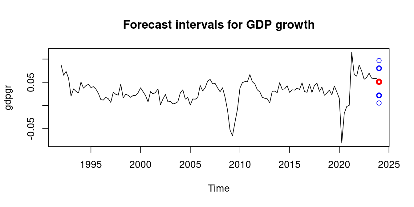
The forecast intervals are quite large, which is not too surprising given the simplicity of the model.
If X_t is a weekly price, then the return (the continuous growth rate) is \log(X_t) - \log(X_{t-1}), which is computed in R as diff(log(X)).
We consider an ADL(4,4) model regressing the weekly gasoline price returns on oil price returns: \begin{align*} gas_t &= \alpha_0 + \alpha_1 gas_{t-1} + \alpha_2 gas_{t-2} + \alpha_3 gas_{t-3} + \alpha_4 gas_{t-4} \\ &+\delta_1 oil_{t-1} + +\delta_2 oil_{t-2} +\delta_3 oil_{t-3} + \delta_4 oil_{t-4} + u_t \end{align*}
We can use the zoo class to assign time points to observations. The base R ts (time series) class can only handle time series with a fixed and regular number of observations per year such as yearly, quarterly, or monthly data. Weekly data do not have exactly the same number of observations per year, which is why we use the more flexible zoo class. zoo is part of the AER package. zoo(mytimeseries, mydates) defines a zooobject.
data(gasoil, package="teachingdata2")
GASOLINE = zoo(gasoil$gasoline, gasoil$date)
BRENT = zoo(gasoil$brent, gasoil$date)
gas = diff(log(GASOLINE))
oil = diff(log(BRENT))
par(mfrow = c(2,2))
plot(GASOLINE, main="Gasoline prices")
plot(BRENT, main="Oil prices")
plot(gas, main="Gasoline returns")
plot(oil, main="Oil returns")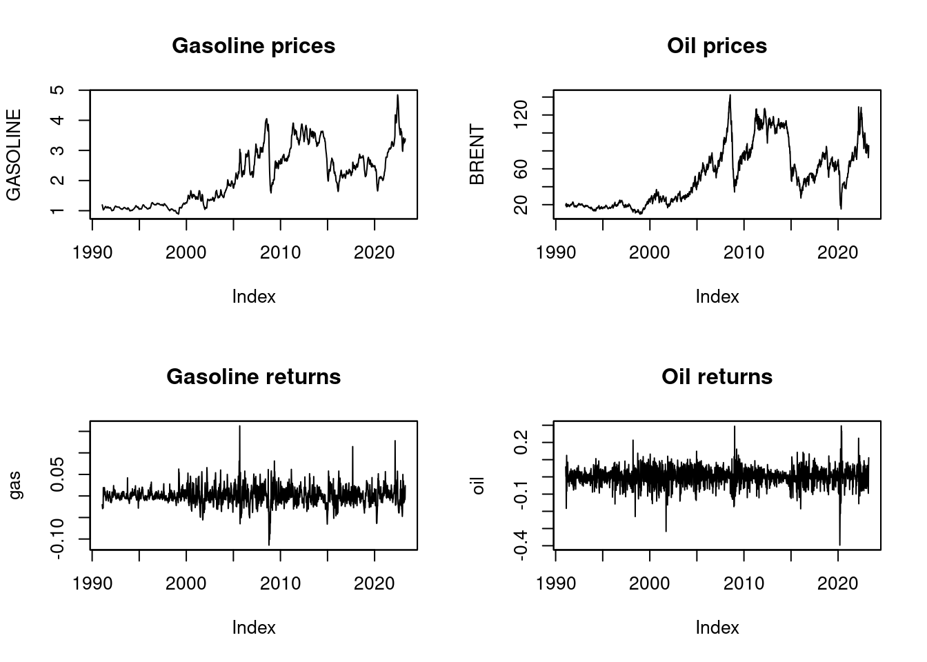
fitADL = dynlm(gas ~ L(gas, 1:4) + L(oil, 1:4))
fitADL
Time series regression with "zoo" data:
Start = 1991-02-25, End = 2023-04-03

Call:
dynlm(formula = gas ~ L(gas, 1:4) + L(oil, 1:4))

Coefficients:
 (Intercept)  L(gas, 1:4)1  L(gas, 1:4)2  L(gas, 1:4)3  L(gas, 1:4)4
   0.0002527     0.3633626     0.0582818     0.0527356    -0.0143211
L(oil, 1:4)1  L(oil, 1:4)2  L(oil, 1:4)3  L(oil, 1:4)4
0.1241477 0.0144996 0.0153132 0.0137106 [,1]
[1,] -0.002331957Consider again the time series regression model of Equation 14.1. Under the regularity condition that the design matrix E[\boldsymbol X_t \boldsymbol X_t'] is invertible (no multicollinearity), the coefficient vector \boldsymbol \beta can be written as \boldsymbol \beta = (E[\boldsymbol X_t \boldsymbol X_t'])^{-1} E[\boldsymbol X_t Y_t]. \qquad \quad \tag{14.3}
In order for \boldsymbol \beta in Equation 14.3 to make sense, it must have same value for all time points t. That is, E[\boldsymbol X_t \boldsymbol X_t'] and E[\boldsymbol X_t Y_t] must be time invariant. To ensure this, we assume that the k+1 vector \boldsymbol Z_t = (Y_t, \boldsymbol X_t')' is stationary.
Recall the definition of stationarity for a multivariate time series:
Stationary univariate time series
A time series Y_t is called stationary if the mean \mu and the autocovariance function \gamma(\tau) do not depend on the time point t. That is, \mu := E[Y_t] < \infty, \quad \text{for all} \ t, and \gamma(\tau) := Cov(Y_t, Y_{t-\tau}) < \infty \quad \text{for all} \ t \ \text{and} \ \tau.
The autocorrelation of order \tau is \rho(\tau) = \frac{Cov(Y_t, Y_{t-\tau})}{Var[Y_t]} = \frac{\gamma(\tau)}{\gamma(0)}, \quad \tau \in \mathbb Z. The autocorrelations of stationary time series typically decay to zero quite quickly as \tau increases, i.e., \rho(\tau) \to 0 as \tau \to \infty. Observations close in time may be highly correlated, but observations farther apart have little dependence.
We define the stationarity concept for multivariate time series analogously:
Stationary multivariate time series
A q-variate time series \boldsymbol Z_t = (Z_{1t}, \ldots, Z_{qt})' is called stationary if each entry Z_{it} of \boldsymbol Z_t is a stationary time series, and, in addition, the cross autocovariances do not depend on t: Cov(Z_{is}, Z_{j,s-\tau}) = Cov(Z_{it}, Z_{j,t-\tau}) < \infty for all \tau \in \mathbb Z and for all s,t = 1, \ldots, T, and i,j = 1, \ldots, q.
The mean vector of \boldsymbol Z_t is \boldsymbol \mu = \big(E[Z_{1t}], \ldots, E[Z_{qt}]\big)' and the autocovariance matrices for \tau \geq 0 are \begin{align*} \Gamma(\tau) &= E[(\boldsymbol Z_t - \boldsymbol \mu) (\boldsymbol Z_{t-\tau} - \boldsymbol \mu)'] \\ &= \begin{pmatrix} Cov(Z_{1,t}, Z_{1,t-\tau}) & \ldots & Cov(Z_{1,t},Z_{q,t-\tau}) \\ \vdots & \ddots & \vdots \\ Cov(Z_{q,t},Z_{1,t-\tau}) & \ldots & Cov(Z_{q,t},Z_{q,t-\tau}) \end{pmatrix} \end{align*}
A time series Y_t is nonstationary if the mean E[Y_t] or the autocovariances Cov(Y_t, Y_{t-\tau}) change with t, i.e., if there exist time points s \neq t with E[Y_t] \neq E[Y_s] \quad \text{or} \quad Cov(Y_t,Y_{t-\tau}) \neq Cov(Y_s,Y_{s-\tau}) for some \tau.
To learn when a time series is stationary and when it is not, it is helpful to study the autoregressive process of order one, AR(1). It is defined as Y_t = \phi Y_{t-1} + u_t, \qquad \quad \tag{14.4} where u_t is an i.i.d. sequence of increments with E[u_t] = 0 and Var[u_t] = \sigma_u^2.
If |\phi| < 1, the AR(1) process is stationary with \mu = 0, \quad \gamma(\tau) = \frac{\phi^\tau \sigma_u^2}{1-\phi^2}, \quad \rho(\tau) = \phi^\tau, \quad \tau \geq 0. Its autocorrelations \rho(\tau) = \phi^\tau decay exponentially in the lag order \tau.
Let’s simulate a stationary AR(1) process. The function filter(u, phi, "recursive") computes Equation 14.4 for parameter phi, a given sequence u and starting value u_0 = 0.
## simulate AR1 with parameter phi=0.8,
## standard normal innovations, and T=400:
set.seed(123)
u = rnorm(400)
AR1 = stats::filter(u, 0.8, "recursive")
par(mfrow = c(1,2))
plot(AR1, main="Simulated AR(1) process")
acf(AR1)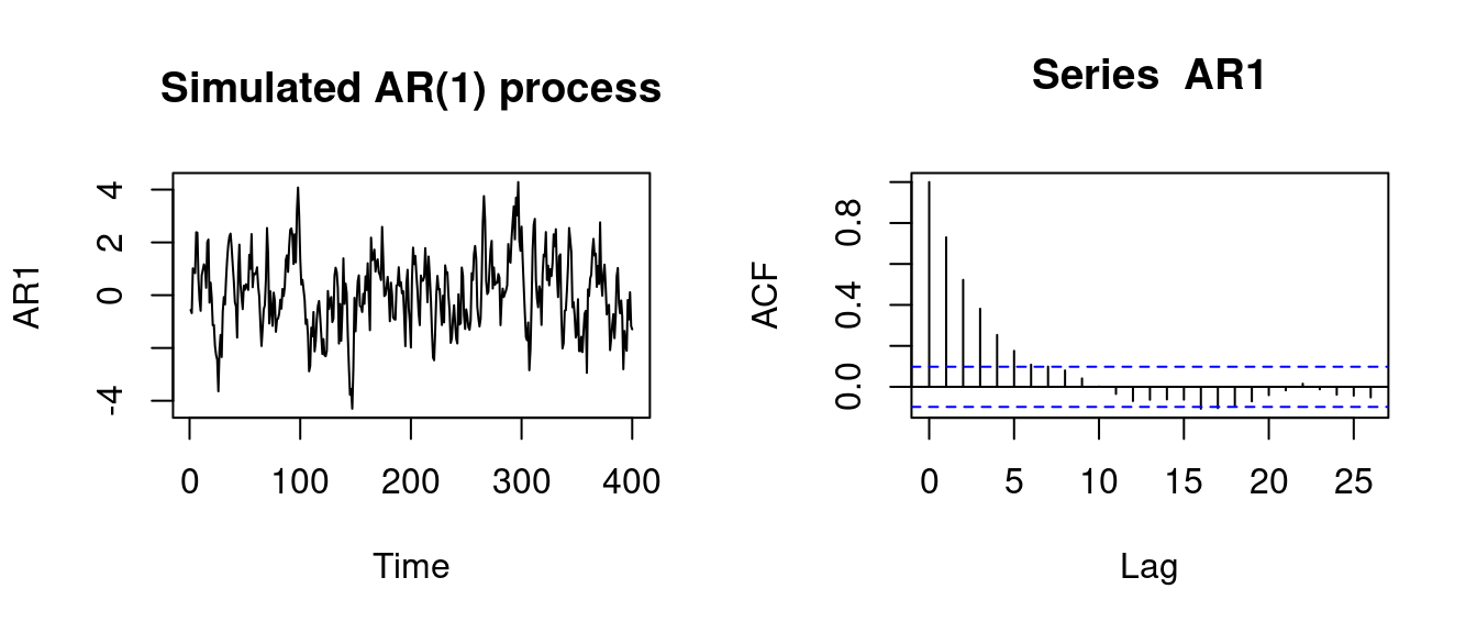
On the right hand side you find the values for the sample autocorrelation function (ACF), which is defined as \widehat \rho(\tau) = \frac{\sum_{t=\tau+1}^T (Y_t - \overline Y) (Y_{t-\tau} - \overline Y)}{\sum_{t=1}^T (Y_t - \overline Y)^2}. The sample autocorrelations of the AR(1) process with parameter \phi = 0.8 converge exponentially to 0 as \tau \to \infty.
The simple random walk is an example of a nonstationary time series process. It is an AR(1) process with \phi=1 and starting value Y_0 = 0, i.e., Y_t = Y_{t-1} + u_t, \quad t \geq 1.
By backward substitution, it can be expressed as the cumulative sum Y_t = \sum_{j=1}^t u_j. It is nonstationary since Cov(Y_t, Y_{t-\tau}) = (t-\tau) \sigma_u^2, which depends on t and becomes larger as t gets larger.
## simulate AR1 with parameter phi=1 (random walk):
RW = stats::filter(u, 1, "recursive")
par(mfrow = c(1,2))
plot(RW, main= "Simulated random walk")
acf(RW)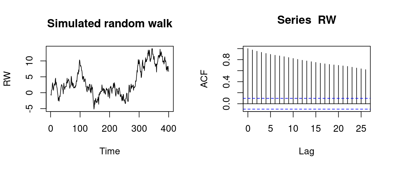
The ACF plots indicate the dynamic structure of the time series and whether they can be regarded as a stationary time series. The ACF of AR1 tends to zero quickly. It can be treated as stationary time series. The ACF of RW tends to zero very slowly, indicating a high persistence. This time series is non-stationary.
data(gdp, package="teachingdata")
par(mfrow = c(2,2))
plot(gdp, main="Nominal GDP Germany")
plot(gdpgr, main = "Annual nominal GDP growth")
acf(gdp)
acf(gdpgr)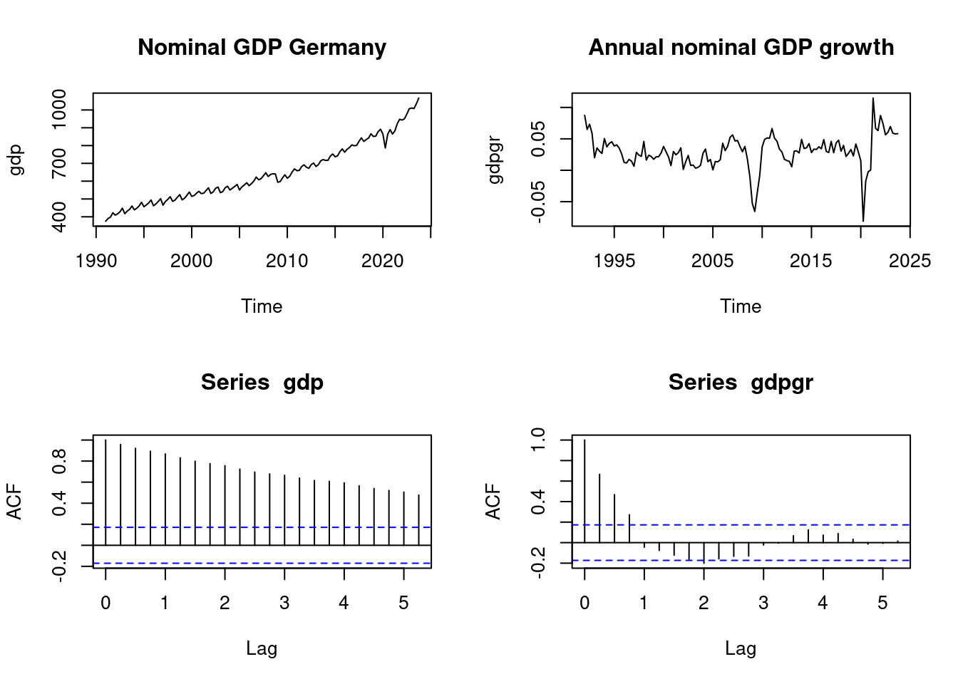
The ACF plots indicate that nominal GDP is nonstationary, while GDP growth is stationary. The asymptotic normality result for OLS is not valid if nonstationary time series are used.