8 Panel Regression
8.1 Panel Data
Panel data is data collected from multiple individuals at multiple points in time.
Individuals in a typical economic panel data application are people, households, firms, schools, regions, or countries. Time periods are often measured in years (annual data), but may have other frequencies.
Y_{it} denotes a variable for individual i at time period t. We index observations by both individuals i = 1, \ldots, n and the time period t = 1, \ldots, T.
Multivariate panel data with k variables can be written as X_{1,it}, \ldots, X_{k,it}, or, in vector form, \boldsymbol X_{it} = \begin{pmatrix} X_{1,it} \\ X_{2, it} \\ \vdots \\ X_{k,it} \end{pmatrix}.
In a balanced panel, each individual i=1, \ldots, n has T observations. The total number of observations is nT. In typical economic panel datasets we have n > T (more individuals than time points) or n \approx T (roughly the same number of individuals as time points).
Often panel data have some missing data for at least one time period for at least one entity. In this case, we call it an unbalanced panel. Notation for unbalanced panels is tedious, so we focus here only on balanced panels. Statistical software can handle unbalanced panel data in much the same way as balanced panel data.
8.2 Pooled Regression
The simplest regression model for panel data is the pooled regression.
Consider a panel dataset with dependent variable Y_{it} and k independent variables X_{1,it}, \ldots, X_{k,it} for i=1, \ldots, n and t=1, \ldots, T.
The first regressor variable represents an intercept (i.e. X_{1,it} = 1). We stack the regressor variables into the k \times 1 vector \boldsymbol X_{it} = \begin{pmatrix} 1 \\ X_{2,it} \\ \vdots \\ X_{k,it} \end{pmatrix}.
The idea of pooled regression is to pool all observations over i=1, \ldots, n and t=1, \ldots, T and run a regression on the combined nT observations.
Pooled Panel Regression Model
The pooled linear panel regression model equation for individual i=1, \ldots, n and time t=1, \ldots, T is Y_{it} = \boldsymbol X_{it}'\boldsymbol \beta + u_{it}, where \boldsymbol \beta = (\beta_1, \ldots, \beta_k)' is the k \times 1 vector of regression coefficients and u_{it} is the error term for individual i at time t.
The pooled OLS estimator is \widehat{\boldsymbol \beta}_{\text{pool}} = \bigg( \sum_{i=1}^n \sum_{t=1}^T \boldsymbol X_{it} \boldsymbol X_{it}' \bigg)^{-1} \bigg( \sum_{i=1}^n \sum_{t=1}^T \boldsymbol X_{it} Y_{it} \bigg).
Similar to linear regression, we can combine the regressors into a pooled regressor matrix of order nT \times k: \boldsymbol X = (\boldsymbol X_{11}, \ldots, \boldsymbol X_{1T}, \boldsymbol X_{21}, \ldots, \boldsymbol X_{2T}, \ldots, \boldsymbol X_{n1}, \ldots, \boldsymbol X_{nT})'. The dependent variable vector is of the order nT \times 1: \boldsymbol Y = (Y_{11}, \ldots, Y_{1T}, Y_{21}, \ldots, Y_{2T}, \ldots, Y_{n1}, \ldots, Y_{nT})'. In matrix notation, the pooled OLS estimator becomes \widehat{\boldsymbol \beta}_{\text{pool}} = (\boldsymbol X' \boldsymbol X)^{-1} \boldsymbol X'\boldsymbol Y.
To illustrate the pooled OLS estimator, consider the Grunfeld dataset, which provides investment, capital stock, and firm value data for 10 firms over 20 years.
  firm year   inv  value capital
1    1 1935 317.6 3078.5     2.8
2    1 1936 391.8 4661.7    52.6
3    1 1937 410.6 5387.1   156.9
4    1 1938 257.7 2792.2   209.2
5    1 1939 330.8 4313.2   203.4
6    1 1940 461.2 4643.9   207.2
fit1 = lm(inv~capital, data=Grunfeld)
fit1
Call:
lm(formula = inv ~ capital, data = Grunfeld)

Coefficients:
(Intercept)      capital
    14.2362       0.4772
In principle, the same assumptions can be made as for the linear regression model. However, in view of (A2), the assumption that (Y_{it}, \boldsymbol X_{it}) is independent of (Y_{i,t-1}, \boldsymbol X_{i,t-1}) is unreasonable because we expect Y_{it} and Y_{i,t-1} to be correlated (autocorrelation) for the same firm i.
This can be seen in the graph below. The observations appear in clusters, with each firm forming a cluster.
plot(inv~capital, col=as.factor(firm), data = Grunfeld)
legend("bottomright", legend=1:10, col=1:10, pch = 1, title="Firm", cex=0.8)
abline(fit1, col = "red")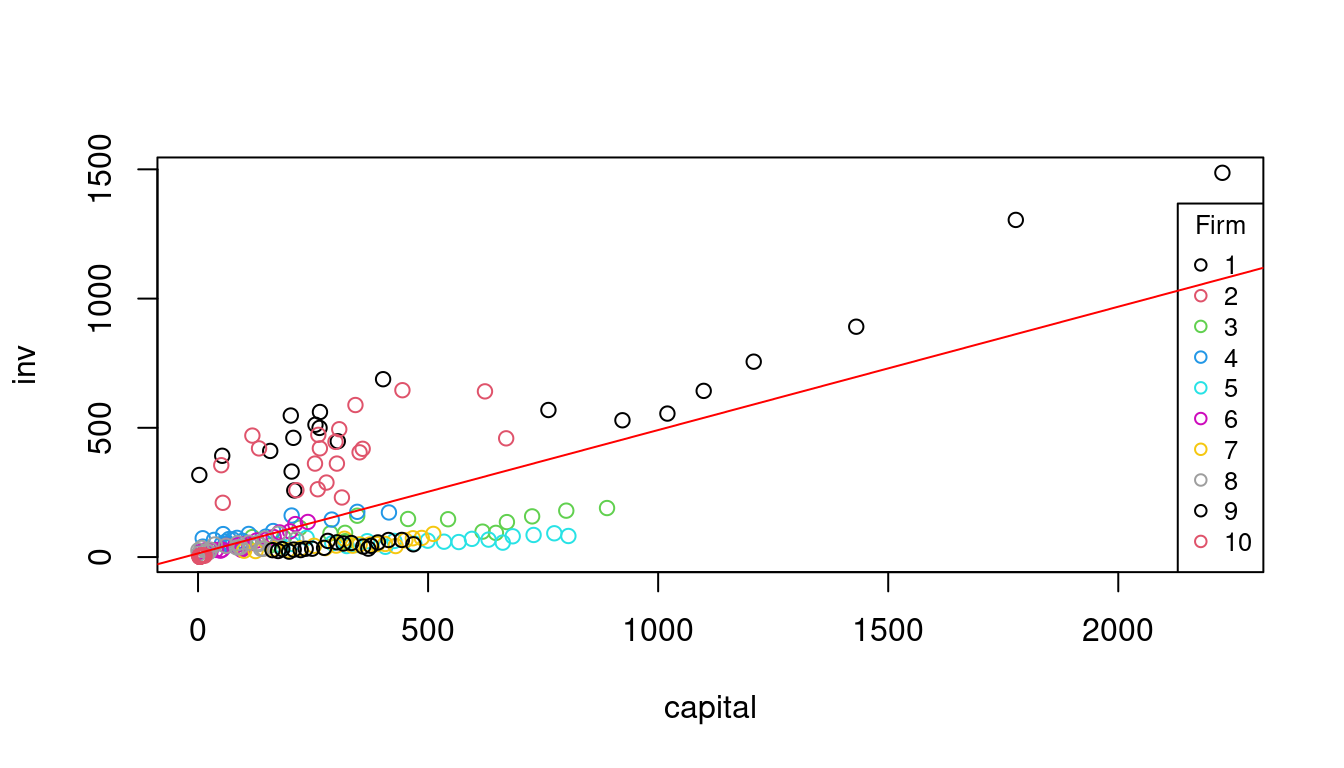
It is still reasonable to assume that the observations of different individuals are independent. For example, if the firms are randomly selected, Y_{it} and Y_{j,t-1} should be independent for i \neq j.
8.3 Pooled Regression Assumptions
We refine our assumptions for the pooled regression case:
(A1-pool) conditional mean independence: E[u_{it} | \boldsymbol X_{i1}, \ldots, \boldsymbol X_{iT}] = 0.
(A2-pool) random sampling: (Y_{i1}, \ldots, Y_{iT}, \boldsymbol X_{i1}', \ldots, \boldsymbol X_{iT}') are i.i.d. draws from their joint population distribution for i=1, \ldots, n.
(A3-pool) large outliers unlikely: 0 < E[Y_{it}^4] < \infty, 0 < E[X_{l,it}^4] < \infty for all l=1, \ldots, k.
(A4-pool) no perfect multicollinearity: \boldsymbol X has full column rank.
Under (A1-pool)–(A4-pool), \widehat{\boldsymbol \beta}_{pool} is consistent for \boldsymbol \beta and asymptotically normal: \frac{\widehat \beta_i - \beta_i}{sd(\widehat \beta_i | \boldsymbol X)} \overset{D}{\to} \mathcal N(0,1) \quad \text{as} \ n \to \infty However, sd(\widehat \beta_i | \boldsymbol X) = \sqrt{Var[\widehat \beta_j | \boldsymbol X]} is different than in the cross-sectional case because of the clustered structure.
The error covariance matrix is of the order nT \times nT and has the block matrix structure \boldsymbol D = Var[\boldsymbol u| \boldsymbol X] = \begin{pmatrix} \boldsymbol D_1 & \boldsymbol 0 & \ldots & \boldsymbol 0 \\ \boldsymbol 0 & \boldsymbol D_2 & \ldots & \boldsymbol 0 \\ \boldsymbol 0 & \boldsymbol 0 & \ddots & \boldsymbol 0 \\ \boldsymbol 0 & \boldsymbol 0 & \ldots & \boldsymbol D_n \end{pmatrix} where \boldsymbol 0 indicates the T \times T matrix of zeros, and on the main diagonal we have the T \times T cluster-specific covariance matrices \boldsymbol D_i = \begin{pmatrix} E[u_{i,1}^2|\boldsymbol X] & E[u_{i,1}u_{i,2}|\boldsymbol X] & \ldots & E[u_{i,1}u_{i,T}|\boldsymbol X] \\ E[u_{i,2}u_{i,1}|\boldsymbol X] & E[u_{i,2}^2|\boldsymbol X] & \ldots & E[u_{i,2}u_{i,T}|\boldsymbol X] \\ \vdots & \vdots & \ddots & \vdots \\ E[u_{i,T}u_{i,1}|\boldsymbol X] & E[u_{i,T} u_{i,2}|\boldsymbol X] & \ldots & E[u_{i,T}^2|\boldsymbol X] \\ \end{pmatrix} for i = 1, \ldots, n.
We have Var[\widehat{ \boldsymbol \beta} | \boldsymbol X] = (\boldsymbol X' \boldsymbol X)^{-1} (\boldsymbol X' \boldsymbol D \boldsymbol X) (\boldsymbol X' \boldsymbol X)^{-1} with \boldsymbol X' \boldsymbol X = \sum_{i=1}^n \sum_{t=1}^T \boldsymbol X_{it} \boldsymbol X_{it}' and \boldsymbol X' \boldsymbol D \boldsymbol X = E\bigg[\sum_{i=1}^n \Big(\sum_{t=1}^T \boldsymbol X_{it} u_{it}\Big)\Big(\sum_{t=1}^T \boldsymbol X_{it} u_{it}\Big)'\Big|\boldsymbol X\bigg]. Therefore, to estimate Var[\widehat{ \boldsymbol \beta} | \boldsymbol X], we need a different estimator than in the cross-sectional case.
The cluster-robust covariance matrix estimator is \boldsymbol{\widehat V}_{\text{pool}} = (\boldsymbol X' \boldsymbol X)^{-1} \sum_{i=1}^N \bigg( \sum_{t=1}^T \boldsymbol X_{it} \widehat u_{it} \bigg) \bigg( \sum_{t=1}^T \boldsymbol X_{it} \widehat u_{it} \bigg)' (\boldsymbol X' \boldsymbol X)^{-1}, which is the cluster-robust analog of the HC0 sandwich estimator. The cluster-robust standard errors are the squareroots of the diagonal entries of \boldsymbol{\widehat V}_{\text{pool}}.
8.4 Pooled Regression Inference
To compute the sandwich form \widehat{\boldsymbol V}_{\text{pool}}, we can use the plm package. It provides the plm() function for estimating linear panel models. The column names of our data frame corresponding to the individual i and the time t are specified by the index option.
library(plm)
fit2 = plm(inv~capital,
           index = c("firm", "year"),
           model = "pooling",
           data=Grunfeld)
fit2
Model Formula: inv ~ capital

Coefficients:
(Intercept)     capital
   14.23620     0.47722
fit2 returns the same estimate as fit1, but is an object of the class plm. You can check it by comparing class(fit1) and class(fit2).
The vcovHC function applied to a plm object returns the cluster-robust covariance matrix \widehat{\boldsymbol V}_{\text{pool}}:
Vpool = vcovHC(fit2)
Vpool
(Intercept) capital
(Intercept) 786.5712535 0.34238311
capital 0.3423831 0.01584317
attr(,"cluster")
[1] "group"coeftest(fit2, vcov. = Vpool)
t test of coefficients:

            Estimate Std. Error t value  Pr(>|t|)
(Intercept) 14.23620   28.04588  0.5076 0.6122959
capital      0.47722    0.12587  3.7914 0.0001988 ***
---
Signif. codes:  0 '***' 0.001 '**' 0.01 '*' 0.05 '.' 0.1 ' ' 1
Alternatively, coeftest(fit2, vcov. = vcovHC) gives the same output. Notice the difference compared to coeftest(fit1, vcov. = vcovHC), which does not take into account the clustered structure in the autocovariance matrix and uses \widehat{\boldsymbol V}_{\text{HC3}}.
Similarly to the cross-sectional case, the functions coefci() and linearHypothesis() can be used for confidence intervals and F/Wald tests.