If two regressors are highly correlated, we can typically drop one of the regressors because they mostly contain the same information.
The idea of principal component regression is to exploit the correlations among the regressors to reduce their number while retaining as much of the original information as possible.
12.1 Principal Components
The principal components (PC) are linear combinations of the regressor variables that capture as much of the variation in the original variables as possible.
Principal Components
Let \boldsymbol X_i be a k-variate vector of regressor variables.
The first principal component is P_{i1} = \boldsymbol w_1'\boldsymbol X_i, where \boldsymbol w_1 satisfies
\boldsymbol w_1 = \argmax_{\boldsymbol w'\boldsymbol w = 1} \ Var[\boldsymbol w' \boldsymbol X_i]
The second principal component is P_{i2} = \boldsymbol w_2'\boldsymbol X_i, where \boldsymbol w_2 satisfies
\boldsymbol w_2 = \argmax_{\substack{\boldsymbol w'\boldsymbol w = 1 \\ \boldsymbol w'\boldsymbol w_1 = 0}} \ Var[\boldsymbol w' \boldsymbol X_i]
The l-th principal component is P_{il} = \boldsymbol w_l'\boldsymbol X_i, where \boldsymbol w_l satisfies
\boldsymbol w_l = \argmax_{\substack{\boldsymbol w'\boldsymbol w = 1 \\ \boldsymbol w'\boldsymbol w_1 = \ldots = \boldsymbol w'\boldsymbol w_{l-1} = 0}} Var[\boldsymbol w' \boldsymbol X_i]
A k-variate regressor vector \boldsymbol X_i has k principal components P_{i1}, \ldots, P_{ik} and k corresponding principal component weights or loadings\boldsymbol w_1, \boldsymbol w_2, \ldots, \boldsymbol w_k.
By definition, the principal components are descendingly ordered by their variance:
Var[P_{i1}] \geq Var[P_{i2}] \geq \ldots \geq Var[P_{ik}] \geq 0
The principal component weights are orthonormal:
\boldsymbol w_i'\boldsymbol w_j = \begin{cases}
1 & \text{if} \ i=j, \\
0 & \text{if} \ i \neq j.
\end{cases}
Moreover, \boldsymbol w_1, \boldsymbol w_2, \ldots, \boldsymbol w_k form an orthonormal basis for the k-dimensional vector space \mathbb R^k. The regressor vector admits the following decomposition into its principal components:
\boldsymbol X_i = \sum_{l=1}^k P_{il} \boldsymbol w_l \qquad \quad
\tag{12.1}
The decomposition of a dataset into its principal components is called principal component analysis (PCA).
12.2 Analytical PCA Solution
In this subsection, we will use some matrix calculus and eigenvalue theory. To recap the relevant matrix algebra, the following resources will be useful:
The maximization problem for the first principal component is
\max_{\boldsymbol w} \ Var[\boldsymbol w' \boldsymbol X_i] \quad \text{subject to} \ \boldsymbol w'\boldsymbol w = 1. \qquad \quad
\tag{12.2} The variance of interest can be rewriten as \begin{align*}
Var[\boldsymbol w' \boldsymbol X_i]
&= E[(\boldsymbol w' (\boldsymbol X_i-E[\boldsymbol X_i]))^2 ] \\
&= E[(\boldsymbol w' (\boldsymbol X_i-E[\boldsymbol X_i]))((\boldsymbol X_i-E[\boldsymbol X_i])' \boldsymbol w) ] \\
&= \boldsymbol w' E[(\boldsymbol X_i-E[\boldsymbol X_i])(\boldsymbol X_i-E[\boldsymbol X_i])']\boldsymbol w \\
&= \boldsymbol w' \Sigma \boldsymbol w
\end{align*} where \Sigma = Var[\boldsymbol X_i] is the population covariance matrix of \boldsymbol X_i. Thus, the constrained maximization problem Equation 12.2 has the Lagrangian
\mathcal L(\boldsymbol w, \lambda) = \boldsymbol w' \Sigma \boldsymbol w - \lambda(\boldsymbol w' \boldsymbol w - 1),
where \lambda is a Lagrange multiplier.
Recall the derivative rules for vectors: If \boldsymbol A is a symmetric matrix, then the derivative of \boldsymbol a' \boldsymbol A \boldsymbol a with respect to \boldsymbol a is 2 \boldsymbol A \boldsymbol a. Therefore, the first order condition with respect to \boldsymbol w is
\Sigma \boldsymbol w = \lambda \boldsymbol w. \qquad \quad
\tag{12.3} The pair (\lambda, \boldsymbol w) must satisfy the eigenequation Equation 12.3. The lagrange multiplier \lambda must be an eigenvalue of \Sigma and the weight vector \boldsymbol w must be a corresponding eigenvector. By the first order condition with respect to \lambda, \boldsymbol w'\boldsymbol w = 1, the eigenvector should be normalized.
Therefore, the variance if interest is
Var[\boldsymbol w' \boldsymbol X_i] = \boldsymbol w' \Sigma \boldsymbol w = \boldsymbol w'(\lambda \boldsymbol w) = \lambda. \qquad \quad
\tag{12.4} Consequently, Var[\boldsymbol w' \boldsymbol X_i] must be an eigenvalue of \Sigma and \boldsymbol w is a corresponding normalized eigenvector.
The expression Var[\boldsymbol w' \boldsymbol X_i] = \lambda is maximized if we use the largest eigenvalue \lambda = \lambda_1. Consequently, the variance of the first principal component P_{i1} is equal to the largest eigenvalue \lambda_1 of \Sigma, and the first principal component weight \boldsymbol w_1 is a normalized eigenvector corresponding to the eigenvalue \lambda_1.
Analogously, the second principal component weight \boldsymbol w_2 must also be a normalized eigenvector of \Sigma with the additional restriction that it is orthogonal to \boldsymbol w_1. Therefore, it cannot be an eigenvector corresponding to the first eigenvalue, and we use the second largest eigenvalue \lambda = \lambda_2 to maximize Equation 12.4.
The variance of the second principal component P_{i2} is equal to the second largest eigenvalue \lambda_2 of \Sigma, and the second principal component weight \boldsymbol w_2 is a corresponding normalized eigenvector.
To continue this pattern, the variance of the l-th principal component P_{il} is equal to the l-th largest eigenvalue \lambda_l of \Sigma, and the l-th principal component weight \boldsymbol w_l is a corresponding normalized eigenvector.
Principal Components Solution
Let \Sigma be the covariance matrix of the k-variate vector of regressor variables \boldsymbol X_i, let \lambda_1 \geq \lambda_2 \geq \ldots \lambda_k \geq 0 be the descendingly ordered eigenvalues of \Sigma, and let \boldsymbol v_1, \ldots, \boldsymbol v_k be corresponding orthonormal eigenvectors.
The principal component weights are \boldsymbol w_l = \boldsymbol v_l for l = 1, \ldots, k
The principal components are P_{il} = \boldsymbol v_l' \boldsymbol X_i, and they have the properties
Var[P_{il}] = \lambda_l, \quad Cov(P_{il}, P_{im}) = 0, \quad l\neq m.
Principal components are uncorrelated because \begin{align*}
Cov(P_{im}, P_{il}) &= E[\boldsymbol w_m'(\boldsymbol X_i - E[\boldsymbol X_i])(\boldsymbol X_i - E[\boldsymbol X_i])' \boldsymbol w_l] \\
&= \boldsymbol w_m' \Sigma \boldsymbol w_l = \lambda_m \boldsymbol w_m' \boldsymbol w_l,
\end{align*} where \boldsymbol w_m' \boldsymbol w_l = 1 if m=l and \boldsymbol w_m' \boldsymbol w_l = 0 if m \neq l
12.3 Sample principal components
The covariance matrix \Sigma = Var[\boldsymbol X_i] is unknown in practice. Instead, we estimate it from the sample \boldsymbol X_1, \ldots, \boldsymbol X_n:
\widehat{\boldsymbol \Sigma} = \frac{1}{n-1} \sum_{i=1}^n (\boldsymbol X_i - \overline{\boldsymbol X})(\boldsymbol X_i - \overline{\boldsymbol X})'.
Let \widehat \lambda_1 \geq \widehat \lambda_2 \geq \ldots, \widehat \lambda_k \geq 0 be the eigenvalues of \widehat{\boldsymbol \Sigma} and let \widehat{\boldsymbol v}_1, \ldots, \widehat{\boldsymbol v}_k be corresponding orthonormal eigenvectors. Then,
The l-th sample principal component for observation i is
\widehat P_{il} = \widehat{\boldsymbol w}_l' \boldsymbol X_i
The l-th sample principal component weight vector is
\widehat{\boldsymbol w}_l = \widehat{\boldsymbol v}_l
The (adjusted) sample variance of the l-th sample principal components series \widehat P_{1l}, \ldots, \widehat P_{nl} is \widehat \lambda_l, and the sample covariances of different principal components series are zero.
12.4 PCA in R
Let’s compute the sample principal components of the mtcars dataset:
pca=prcomp(mtcars)## the principal components are arranged by columnspca$x|>head()
Principal components are sensitive to the scaling of the data. Consequently, it is recommended to first scale each variable in the dataset to have mean zero and unit variance: scale(mtcars). In this case, \Sigma is the correlation matrix.
Since the sample principal components are uncorrelated, the total variation in the data is
Var\bigg[\sum_{m=1}^k \widehat P_{im}\bigg] = \sum_{m=1}^k Var[\widehat P_{im}] = \sum_{m=1}^k \widehat \lambda_l.
The proportion of variance explained by the l-th principal component is
\frac{Var[\widehat P_{il}]}{Var[\sum_{m=1}^k \widehat P_{im}]} = \frac{\widehat \lambda_l}{\sum_{m=1}^k \widehat \lambda_m}
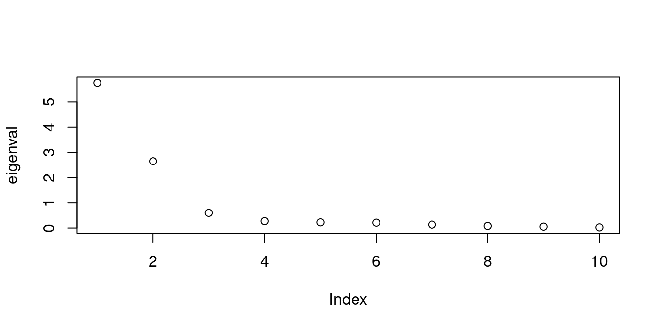
A scree plot is useful to see how much each principal component contributes to the total variation:
The first principal component explains more that 60% of the variation, the first four explain more than 90% of the variation, the first 6 more than 95%, and the first 9 principal component more than 99% of the variation.
12.6 Linear regression with principal components
Principal components can be used to estimate the high-dimensional (large k) linear regression model
Y_i = \boldsymbol X_i' \boldsymbol \beta + u_i, \quad i=1, \ldots, n.
Since the principal component weights \boldsymbol w_1, \ldots, \boldsymbol w_k form a basis of \mathbb R^k, the regressors have the basis representation given by Equation 12.1. Similarly, we can represent the coefficient vector in terms of the principal component basis:
\boldsymbol \beta = \sum_{l=1}^k \theta_l \boldsymbol w_l, \quad \theta_l = \boldsymbol w_l'\boldsymbol \beta. \qquad \quad
\tag{12.5} Inserting in the regression function gives
\boldsymbol X_i' \boldsymbol \beta = \sum_{l=1}^k \underbrace{\boldsymbol X_i'\boldsymbol w_l}_{=P_{il}} \theta_l,
and the regression equation becomes
Y_i = \sum_{l=1}^k P_{il} \theta_l + u_i.
\tag{12.6} This regression equation is convenient because the regressors P_{il} are uncorrelated, and OLS estimates for \theta_l can be inserted back into Equation 12.5 to get an estimate for \boldsymbol \beta.
When k is large, this approach is still prone to overfitting. The k principal components of \boldsymbol X_i explain 100% of its variance, but it may be reasonable to select a smaller number of principal components p < k that explain 95% or 99% of the variance.
The remaining k-p principal components explain only 5% or 1% of the variance. The idea is that we truncate the model by assuming that the remaining principal components contain only noise that is uncorrelated with Y_i.
Assumption (PC): E[P_{im} Y_i] = 0 for all m = p+1, \ldots, k.
Because the principal components are uncorrelated, we have \theta_l = E[Y_i P_{il}]/E[P_{il}^2], and, therefore \theta_m = 0 for m = p+1, \ldots, k. Consequently,
\boldsymbol \beta = \sum_{l=1}^p \theta_l \boldsymbol w_l, \qquad \quad
\tag{12.7} and Equation 12.6 becomes a factor model with p factors:
Y_i = \sum_{l=1}^p \theta_l P_{il} + u_i = \boldsymbol P_i' \boldsymbol \theta + u_i,
where \boldsymbol P_i = (P_{i1}, \ldots, P_{ip})' and \boldsymbol \theta = (\theta_1, \ldots, \theta_p)'. The least squares estimator of \boldsymbol \theta using the regressors \boldsymbol P_i, i=1, \ldots n can then be inserted to Equation 12.7 to obtain an estimate for \boldsymbol \beta.
In practice, the principal components are unknown and must be replaced by the first p sample principal components
\widehat{\boldsymbol P}_i = (\widehat P_{i1}, \ldots, \widehat P_{ip})', \quad \widehat P_{il} = \widehat{\boldsymbol w}_l'\boldsymbol X_i.
The feasible least squares estimator for \theta is
\widehat{\boldsymbol \theta} = (\widehat \theta_1, \ldots, \widehat \theta_p)' = \bigg( \sum_{i=1}^n \widehat{\boldsymbol P}_i \widehat{\boldsymbol P}_i'\bigg)^{-1} \sum_{i=1}^n \widehat{\boldsymbol P}_i Y_i,
and the principal components estimator for \boldsymbol \beta is
\widehat{\boldsymbol \beta}_{pc} = \sum_{l=1}^p \widehat \theta_l \widehat{\boldsymbol w}_l.
12.7 Selecting the number of factors
To select the number of principal components, one practical approach is to choose those that explain a pre-specified percentage (90-99%) of the total variance.
Y=mtcars$mpgX=model.matrix(mpg~., data =mtcars)[,-1]|>scale()## principal component analysispca=prcomp(X)P=pca$x#full matrix of all principal components## variance explainedeigenval=pca$sdev^2varexpl=eigenval/sum(eigenval)cumsum(varexpl)
The first four principal components explain more than 92% of the variance, and the first seven more than 98%.
Another method involves creating a scree plot to display the eigenvalues (variances) for each principal component and identifying the point where the eigenvalues sharply drop (elbow point).
Selecting the number of principal components, similar to shrinkage estimation, involves balancing variance and bias. If the Assumption (PC) holds, the PC estimator is unbiased; if it doesn’t, a small bias is introduced. Increasing the number of components p reduces bias but increases variance, while decreasing p reduces variance but increases bias.
Similarly to the shrinkage parameter in ridge and lasso estimation, the number of factors p can be treated as a tuning parameter. We can use m-fold cross validation to select p such that the MSE is minimized.