7 Regression Diagnostics
This section discusses some graphical and analytical regression diagnostic techniques for detecting outliers and assessing whether the assumptions of our regression model are met.
7.1 Leverage values
Leverage values h_{ii} indicate how much influence an observation \boldsymbol X_i has on the regression fit. They are calculated as h_{ii} = \boldsymbol X_i' (\boldsymbol X' \boldsymbol X)^{-1} \boldsymbol X_i and represent the diagonal entries of the hat-matrix \boldsymbol P = \boldsymbol X (\boldsymbol X' \boldsymbol X)^{-1} \boldsymbol X'.
A low leverage implies the presence of many regressor observations similar to \boldsymbol X_i in the sample, while a high leverage indicates a lack of similar observations near \boldsymbol X_i.
An observation with a high leverage h_{ii} but a response value Y_i that is close to the true regression line \boldsymbol X_i' \boldsymbol \beta (indicating a small error u_i) is considered a good leverage point. It positively influences the model, especially in data-sparse regions.
Conversely, a bad leverage point occurs when both h_{ii} and the error u_i are large, indicating both unusual regressor and response values. This can misleadingly impact the regression fit.
The actual error term is unknown, but standardized residuals can be used to differentiate between good and bad leverage points.
7.2 Standardized residuals
Many regression diagnostic tools rely on the residuals of the OLS estimation \widehat u_i because they provide insight into the properties of the unknown error terms u_i.
Under the homoskedastic linear regression model (A1)–(A5), the errors are independent and have the property Var[u_i | \boldsymbol X] = \sigma^2. Since \boldsymbol P \boldsymbol X = \boldsymbol X and, therefore, \widehat{\boldsymbol u} = (\boldsymbol I_n - \boldsymbol P)\boldsymbol Y = (\boldsymbol I_n - \boldsymbol P)(\boldsymbol X\boldsymbol \beta + \boldsymbol u) = (\boldsymbol I_n - \boldsymbol P)\boldsymbol u, the residuals have a different property: Var[\widehat{\boldsymbol u} | \boldsymbol X] = \sigma^2 (\boldsymbol I_n - \boldsymbol P). The i-th residual satisfies Var[\widehat u_i | \boldsymbol X] = \sigma^2 (1 - h_{ii}), where h_{ii} is the i-th leverage value.
Under the assumption (A5), the variance of \widehat u_i depends on \bold X, while the variance of u_i does not. Dividing by \sqrt{1-h_{ii}} removes the dependency: Var\bigg[ \frac{\widehat u_i}{\sqrt{1-h_{ii}}} \bigg| \boldsymbol X\bigg] = \sigma^2
The standardized residuals are defined as follows: r_i := \frac{\widehat u_i}{\sqrt{s_{\widehat u}^2 (1-h_{ii})}}.
Standardized residuals are available using the R command rstandard().
7.3 Diagnostics plots
Let’s consider the CASchools dataset from the previous subsection:
The plot() function applied to an lm object returns four diagnostics plots:
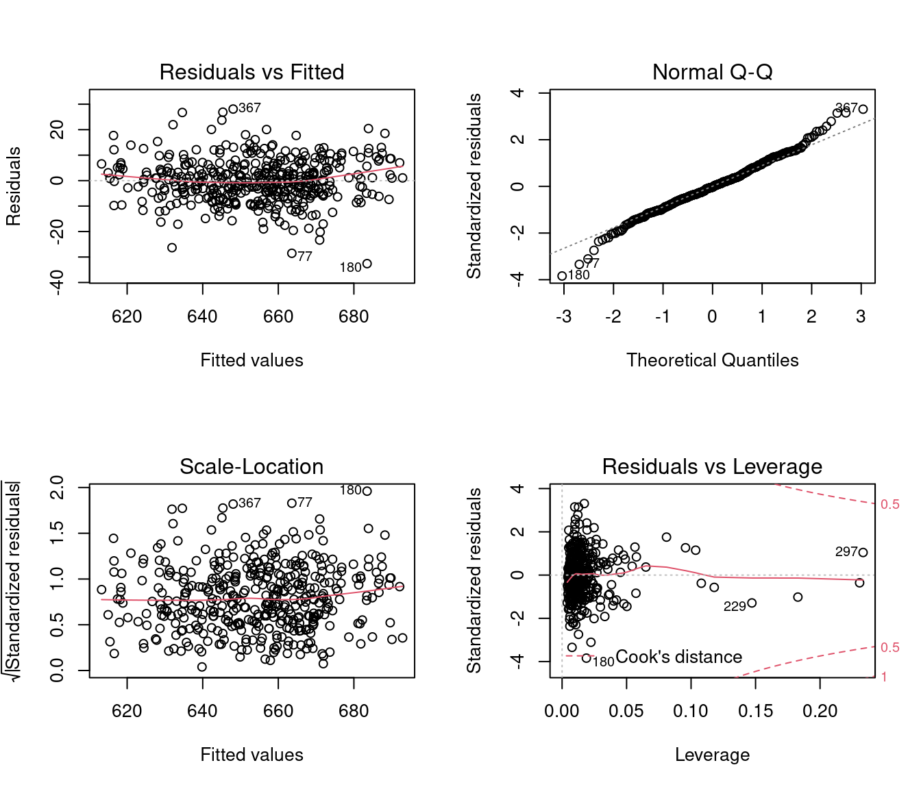
These plots show different scatterplots of the fitted values \widehat Y_i, residuals \widehat u_i, quantiles of the standard normal distribution, leverage values, and standardized residuals.
The red solid line indicates a local scatterplot smoother, which is a smooth locally weighted line through the points on the scatterplot to visualize the general pattern of the data.
Plot 1: Residuals vs Fitted
This plot indicates whether there are strong hidden nonlinear relationships between the response and the regressors that are not captured by the model. If a linear model is estimated but the relationship is nonlinear, then the assumption (A1) E[u_i \mid \boldsymbol X_i] = 0 is violated.
The residuals serve as a proxy for the unknown error terms. If you find equally spread residuals around a horizontal line without distinct patterns, that is a good indication you don’t have non-linear relationships.
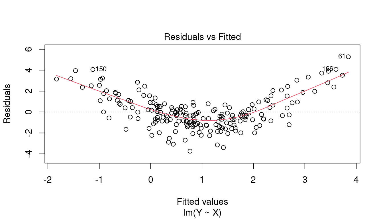
In the CASchools regression, there is only little indication for an omitted non-linear relationship. Here is an example of a strong omitted nonlinear pattern:
Plot 2: Normal Q-Q
The QQ plot is a graphical tool to help us assess if the errors are conditionally normally distributed, i.e. whether assumption (A6) is satisfied.
Let r_{(i)} be the order statistics of the standardized residuals (sorted standardized residuals). The QQ plot plots the ordered standardized residuals u_{(i)}^* against the ((i-0.5)/n)-quantiles of the standard normal distribution.
If the residuals are lined well on the straight dashed line, there is indication that the distribution of the residuals is close to a normal distribution.
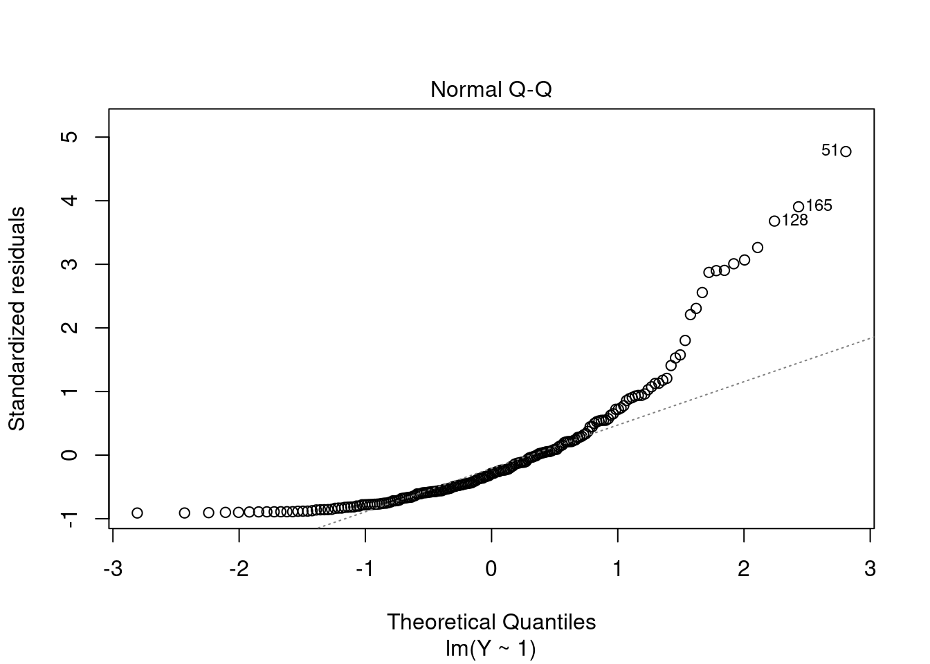
In the CASchools regression, we see a slight deviation from normality in the tails. Here is an extrem example with a strong deviation from normality:
Plot 3: Scale-Location
This plot shows if error terms are spread equally along the ranges of regressor values, which is how you can check the assumption of homoskedasticity (A5).
If you see a horizontal line with equally spread points, there is no indication for heteroskedasticity.
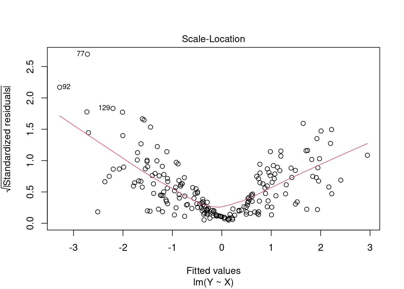
In the CASchools regression, we have some indication for weak heteroskedasticity. Here is an example with extreme heteroskedasticity:
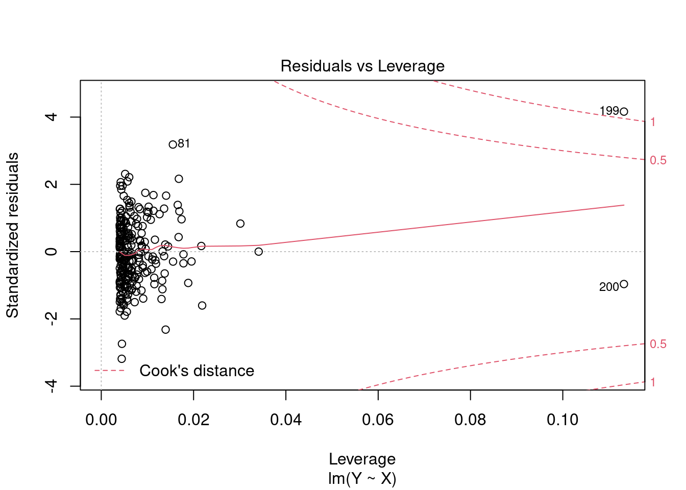
Plot 4: Residuals vs Leverage
Plotting standardized residuals against leverage values provides a graphical tool for detecting outliers. High leverage points have a strong influence on the regression fit. High leverage values with standardized residuals close to 0 are good leverage points, and high leverage values with large standardized residuals are bad leverage points.
The plot also shows Cook’s distance thresholds. Cook’s distance for observation i is defined as D_i = \frac{(\widehat{\boldsymbol \beta}_{(-i)} - \widehat{\boldsymbol \beta})' \boldsymbol X' \boldsymbol X (\widehat{\boldsymbol \beta}_{(-i)} - \widehat{\boldsymbol \beta})}{k s_{\widehat u}^2}, where \widehat{\boldsymbol \beta}_{(-i)} = \widehat{\boldsymbol \beta} - (\boldsymbol X' \boldsymbol X)^{-1} \boldsymbol X_i \widehat u_i (1-h_{ii})^{-1} is the i-th leave-one-out estimator (the OLS estimator when the i-th observation is left out).
We should pay special attention to points outside Cook’s distance thresholds of 0.5 and 1 and check for measurement errors or other anomalies.
Here is an example with two high leverage points. Observation i=200 is a good leverage point and i=199 is a bad leverage point:
7.4 Diagnostics tests
The asymptotic properties of the OLS estimator and inferential methods using HC-type standard errors do not depend on the validity of the homoskedasticity and normality assumptions (A5)–(A6).
However, if you are interested in exact inference, verifying the assumptions (A5)–(A6) becomes crucial, especially in small samples.
7.4.1 Breusch-Pagan Test (Koenker’s version)
Under homoskedasticity, the variance of the error term does not depend on the values of the regressors.
To test for heteroskedasticity, we regress the squared residuals on the regressors. \widehat u_i^2 = \boldsymbol X_i' \boldsymbol \gamma + v_i, \quad i=1, \ldots, n. \tag{7.1} Here, \boldsymbol \gamma are the auxiliary coefficients and v_i are the auxiliary error terms. Under homoskedasticity, the regressors should not be able to explain any variation in the residuals.
Let R^2_{aux} be the r-squared coefficient of the auxiliary regression of Equation 7.1. The test statistic: BP = n R^2_{aux} Under the null hypothesis of homoskedasticity, we have BP \overset{D}{\to} \chi^2_{k-1} Test decision rule: Reject H_0 if BP exceeds \chi^2_{(1-\alpha,k-1)}.
In R we can apply the bptest() function from the lmtest package to the lm object of our regression.
7.4.2 Jarque-Bera Test
A general property of any normally distributed random variable is that it has a skewness of 0 and a kurtosis of 3.
Under (A5)–(A6), we have u_i \sim \mathcal N(0,\sigma^2), which implies E[u_i^3] = 0 and E[u_i^4] = 3 \sigma^4.
Consider the sample skewness and the sample kurtosis of the residuals from your regression: \widehat{skew}_{\widehat u} = \frac{1}{n \widehat \sigma_{\widehat u}^3} \sum_{i=1}^n \widehat u_i^3, \quad \widehat{kurt}_{\widehat u} = \frac{1}{n \widehat \sigma_{\widehat u}^4} \sum_{i=1}^n \widehat u_i^4
Jarque-Bera test statistic and null distribution if (A5)–(A6) hold: JB = n \bigg( \frac{1}{6} \big(\widehat{skew}_{\widehat u}\big)^2 + \frac{1}{24} \big(\widehat{kurt}_{\widehat u} - 3\big)^2 \bigg) \overset{D}{\to} \chi^2_2. Test decision rule: Reject the null hypothesis of normality if JB exceeds \chi^2_{(1-\alpha,2)}.
The Jarque-Bera test is sensitive to outliers.
In R we apply use the jarque.test() function from the moments package to the residual vector from our regression.