6 Case Study I: Score Data
6.1 Data Set Description
The California School data set (CASchools) is included in the R package AER. This dataset contains information on various characteristics of schools in California, such as test scores, teacher salaries, and student demographics.
Upon examination we find that the dataset contains mostly numeric variables, but it lacks two important ones we’re interested in: average test scores and student-teacher ratios. However, we can calculate them using the available data.
To find the student-teacher ratio, we divide the total number of students by the number of teachers. For the average test score, we just need to average the math and reading scores. In the next code chunk, we’ll demonstrate how to create these variables as vectors and add them to the CASchools dataset.
# compute student-teacher ratio and append it to CASchools
CASchools$STR <- CASchools$students/CASchools$teachers

# compute test score and append it to CASchools
CASchools$score <- (CASchools$read + CASchools$math)/2
If we ran summary(CASchools) again we would find the two variables of interest as additional variables named STR and score.
6.2 Linear Regression
Let’s suppose we were interested in the following regression model
TestScore = \beta_0 + \beta_1 \, STR + \beta_2 \, english + u
In this regression, we aim to explore how test scores (score) are influenced by student-teacher ratio (STR) and the percentage of English learners (english). The variable english indicates the proportion of students who may require additional support or resources to improve their English language skills within each school.
We would run this model in R using the lm() function and explore the regression estimates with coeftest().
# run the model
model <- lm(score ~ STR + english, data = CASchools)
# report estimates
coeftest(model, vcov. = vcovHC)
t test of coefficients:

              Estimate Std. Error  t value Pr(>|t|)
(Intercept) 686.032245   8.812242  77.8499  < 2e-16 ***
STR          -1.101296   0.437066  -2.5197  0.01212 *
english      -0.649777   0.031297 -20.7617  < 2e-16 ***
---
Signif. codes:  0 '***' 0.001 '**' 0.01 '*' 0.05 '.' 0.1 ' ' 1
The coeftest() function in R, along with suitable options such as vcov. = vcovHC for robust standard errors, automatically includes statistics such as standard errors, t-statistics, and p-values, which is exactly what we need to test hypotheses about single coefficients (\beta_j) in regression models.
We can also compute confidence intervals for individual coefficients in the multiple regression model by using the function coefci(). This function computes confidence intervals at the 95% level by default.
# compute confidence intervals for all coefficients in the model
coefci(model, vcov. = vcovHC)
2.5 % 97.5 %
(Intercept) 668.7102930 703.3541961
STR -1.9604231 -0.2421682
english -0.7112962 -0.5882574To obtain confidence intervals at a different level, say 90%, we set the argument level in our call of coefci() accordingly.
coefci(model, vcov. = vcovHC, level = 0.9) 5 % 95 %
(Intercept) 671.5051238 700.5593652
STR -1.8218062 -0.3807851
english -0.7013703 -0.5981834The output above shows that zero is not an element of the confidence interval for the coefficient on STR, so we can reject the null hypothesis at significance levels of 5\% and 10\% (Note that rejection at the 5\% level implies rejection at the 10\% level anyway).
We can bring this conclusion further via the p-value for STR: 0.01 < 0.01212<0.05, which indicates that this coefficient estimate is significant at the 5\% level but not at the 1\% level.
6.3 Bad Controls
Let’s suppose now that we are interested in investigating the average effect on test scores of reducing the student-teacher ratio when the expenditures per pupil and the percentage of english learning pupils are held constant.
Let us augment our model by an additional regressor expenditure, that is a measure for the total expenditure per pupil in the district. For this model, we will include expenditure as measured in thousands of dollars. Our new model would be
TestScore = \beta_0 + \beta_1 \, STR + \beta_2 \, english + \beta_3 \, expenditure + u
Let us now estimate the model:
# scale expenditure to thousands of dollars
CASchools$expenditure <- CASchools$expenditure/1000

# estimate the model
model <- lm(score ~ STR + english + expenditure, data = CASchools)
coeftest(model, vcov. = vcovHC)
t test of coefficients:

              Estimate Std. Error  t value Pr(>|t|)
(Intercept) 649.577947  15.668623  41.4572  < 2e-16 ***
STR          -0.286399   0.487513  -0.5875  0.55721
english      -0.656023   0.032114 -20.4278  < 2e-16 ***
expenditure   3.867901   1.607407   2.4063  0.01655 *
---
Signif. codes:  0 '***' 0.001 '**' 0.01 '*' 0.05 '.' 0.1 ' ' 1
The estimated impact of a one-unit change in the student-teacher ratio on test scores, while holding expenditure and the proportion of English learners constant, is -0.29. It is much smaller than the estimated coefficient in our initial model where we didn’t include expenditure.
Additionally, this coefficient of STR is no longer statistically significant, even at a 10\% significance level, as indicated by a p-value of 0.56. This lack of significance for \beta_1 may stem from a larger standard error resulting from the inclusion of expenditure in the model, leading to less precise estimation of the coefficient on STR. This scenario highlights the challenge of dealing with strongly correlated predictors.
Note that expenditure can be classified as a bad control because higher expenditure per pupil may be the cause of a decrease in the student-teacher ratio. By adding expenditure to the regression we are controlling away our causal effect of STR on score.
The correlation between STR and expenditure can be determined using the cor() function.
# compute the sample correlation between 'STR' and 'expenditure'
cor(CASchools$STR, CASchools$expenditure)
[1] -0.6199822This indicates a moderately strong negative correlation between the two variables.
The estimated model is
\widehat{TestScore} = \underset{(15.67)}{649.58} \,- \underset{(0.49)}{0.29} \, STR - \underset{(0.03)}{0.66} \, english + \underset{(1.61)}{3.87} \, expenditure Could we reject the hypothesis that both the STR coefficient and the expenditure coefficient are zero? To answer this, we need to conduct joint hypothesis tests, which involve placing restrictions on multiple regression coefficients. This differs from individual t-tests, where restrictions are applied to a single coefficient.
To test whether both coefficients are zero, we will conduct a heteroskedasticity-robust F-test. To do this in R, we can use the function waldtest() contained in the package lmtest.
Wald test

Model 1: score ~ STR + english + expenditure
Model 2: score ~ english
  Res.Df Df      F   Pr(>F)
1    416
2    418 -2 5.2617 0.005537 **
---
Signif. codes:  0 '***' 0.001 '**' 0.01 '*' 0.05 '.' 0.1 ' ' 1
The output reveals that the F-statistic for this joint hypothesis test is 5.26 and the corresponding p-value is about 0.0055. We can therefore reject the null hypothesis that both coefficients are zero at the 1\% level of significance. Notice that the individual t-tests for STR and expenditure are insignificant at the 1\% level.
6.4 Good Controls
In order to reduce the risk of omitted variable bias, it is essential to include control variables in regression models. In our case, we are interested in estimating the causal effect of a change in the student-teacher ratio on test scores.
By including english as control variable, we aimed to control for unobservable student characteristics which correlate with the student-teacher ratio and are assumed to have an impact on test score. Including expenditure was actually not a good idea because it is highly correlated with STR (imperfect multicollinearity) and may be the cause of the student-teacher ratio (bad control).
There are other interesting control variables to observe:
lunch: the share of students that qualify for a subsidized or even a free lunch at school.calworks: the percentage of students that qualify for the CalWorks income assistance program.
Students eligible for CalWorks live in families with a total income below the threshold for the subsidized lunch program, so both variables are indicators for the share of economically disadvantaged children. We suspect both indicators are highly correlated.
# estimate the correlation between 'calworks' and 'lunch'
cor(CASchools$calworks, CASchools$lunch)
[1] 0.7394218If they are highly correlated as we just confirmed, there is no standard way to proceed when deciding which variable to use. It may not be a good idea to use both variables as regressors in view of collinearity, but as long as we are only interested in the coefficient of STR we do not care whether the coefficients of calworks and lunch have an imperfect multicollinearity problem.
Let’s first explore further these control variables and how they correlate with the dependent variable by plotting them against test scores.
correlations = round(cor(CASchools$score, CASchools |>
                           select(english, lunch, calworks)),2)
par(mfrow = c(1,3), pch = 20, col = "steelblue", bty="n")
plot(score ~ english, data = CASchools, xlim = c(0, 100),
     main = paste("cor =",correlations[1]))
plot(score ~ lunch, data = CASchools, xlim = c(0, 100),
     main = paste("cor =",correlations[2]))
plot(score ~ calworks, data = CASchools, xlim = c(0, 100),
     main = paste("cor =",correlations[3]))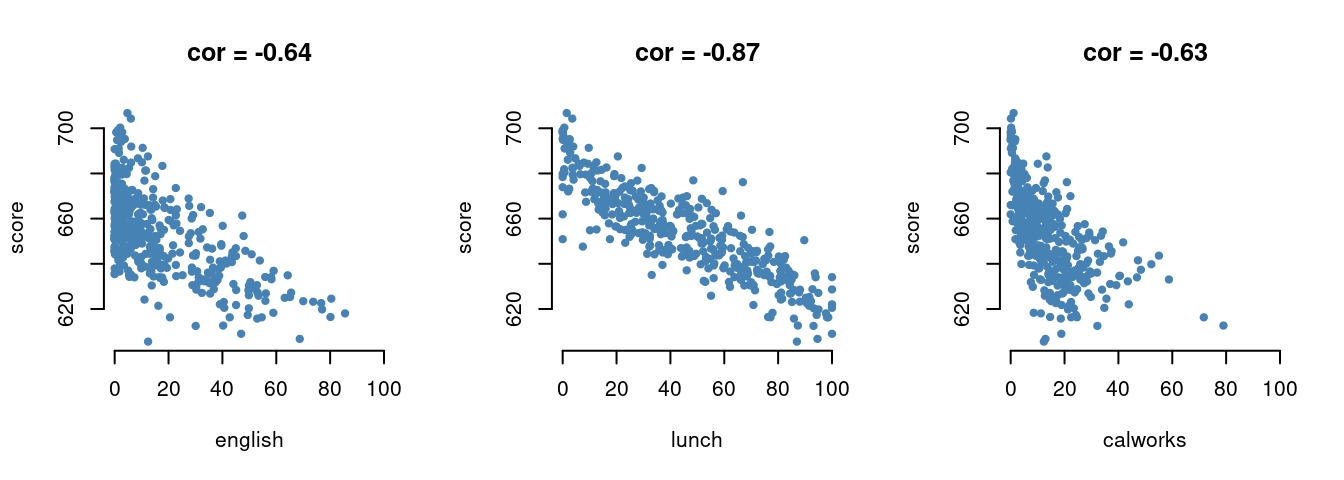
We shall consider five different model equations:
\begin{align} \text{TestScore} &= \beta_0 + \beta_1 \, \text{STR} + u, \\ \text{TestScore} &= \beta_0 + \beta_1 \, \text{STR} + \beta_2 \, \text{english} + u, \\ \text{TestScore} &= \beta_0 + \beta_1 \, \text{STR} + \beta_2 \, \text{english} + \beta_3 \, \text{lunch} + u, \\ \text{TestScore} &= \beta_0 + \beta_1 \, \text{STR} + \beta_2 \, \text{english} + \beta_4 \, \text{calworks} + u, \\ \text{TestScore} &= \beta_0 + \beta_1 \, \text{STR} + \beta_2 \, \text{english} + \beta_3 \, \text{lunch} + \beta_4 \, \text{calworks} + u. \end{align}
The best way to report regression results is in a table. The stargazer package is very convenient for this purpose. It provides a function that generates professionally looking HTML and LaTeX tables that satisfy scientific standards. One simply has to provide one or multiple object(s) of class lm. The rest is done by the function stargazer().
# estimate different model specifications
spec1 <- lm(score ~ STR, data = CASchools)
spec2 <- lm(score ~ STR + english, data = CASchools)
spec3 <- lm(score ~ STR + english + lunch, data = CASchools)
spec4 <- lm(score ~ STR + english + calworks, data = CASchools)
spec5 <- lm(score ~ STR + english + lunch + calworks, data = CASchools)

# gather robust standard errors in a list
rob_se <- list(sqrt(diag(vcovHC(spec1))),
               sqrt(diag(vcovHC(spec2))),
               sqrt(diag(vcovHC(spec3))),
               sqrt(diag(vcovHC(spec4))),
sqrt(diag(vcovHC(spec5))))stargazer(spec1, spec2, spec3, spec4, spec5,
se = rob_se,
type="html",
omit.stat = "f")| Dependent variable: | |||||
| score | |||||
| (1) | (2) | (3) | (4) | (5) | |
| STR | -2.280*** | -1.101** | -0.998*** | -1.308*** | -1.014*** |
| (0.524) | (0.437) | (0.274) | (0.343) | (0.273) | |
| english | -0.650*** | -0.122*** | -0.488*** | -0.130*** | |
| (0.031) | (0.033) | (0.030) | (0.037) | ||
| lunch | -0.547*** | -0.529*** | |||
| (0.024) | (0.039) | ||||
| calworks | -0.790*** | -0.048 | |||
| (0.070) | (0.062) | ||||
| Constant | 698.933*** | 686.032*** | 700.150*** | 697.999*** | 700.392*** |
| (10.461) | (8.812) | (5.641) | (7.006) | (5.615) | |
| Observations | 420 | 420 | 420 | 420 | 420 |
| R2 | 0.051 | 0.426 | 0.775 | 0.629 | 0.775 |
| Adjusted R2 | 0.049 | 0.424 | 0.773 | 0.626 | 0.773 |
| Residual Std. Error | 18.581 (df = 418) | 14.464 (df = 417) | 9.080 (df = 416) | 11.654 (df = 416) | 9.084 (df = 415) |
| Note: | p<0.1; p<0.05; p<0.01 | ||||
Each column in this table contains most of the information provided also by coeftest() and summary() for each of the models under consideration. Each of the coefficient estimates includes its standard error in parenthesis and one, two or three asterisks representing their significance levels (10% , 5% and 1%). Although t-statistics are not reported, one may compute them manually simply by dividing a coefficient estimate by the corresponding standard error. At the bottom of the table summary statistics for each model and a legend are reported.
From the model comparison we observe that including control variables approximately cuts the coefficient on STR in half. Additionally, the estimation seems to remain unaffected by the specific set of control variables employed. Thus, the inference drawn is that, under all other conditions held constant, reducing the student-teacher ratio by one unit is associated with an estimated average rise in test scores of roughly 1 point.
Incorporating student characteristics as controls increased both R^2 and \bar{R^2} from about 0.05 (spec1) to about 0.77 (spec3 and spec5), indicating these variables’ suitability as predictors for test scores.
We also observe that the coefficients for some of the control variables are not significant in some models. For example in spec5, the coefficient on calworks is not significantly different from zero at the 10\% level.
Lastly, we see that the effect on the estimate (and its standard error) of the coefficient on STR when adding calworks to the base specification spec3 is minimal. Hence, we can identify calworks as an unnecessary control variable, especially considering the incorporation of lunch in this model.
6.5 Nonlinear Specifications
Sometimes a nonlinear regression function is better suited for estimating a population relationship. Let’s have a look at an example that explores the relationship between the income of schooling districts and their test scores.
We start our analysis by computing the correlation between both variables.
cor(CASchools$income, CASchools$score)[1] 0.7124308Income and test score are positively correlated: school districts with above-average income tend to achieve above-average test scores. But does a linear regression adequately model the data? To investigate this further, let’s visualize the data by plotting it and adding a linear regression line.
# Fit a simple linear model and plot observations with the regression line
linear_model <- lm(score ~ income, data = CASchools)
plot(CASchools$income, CASchools$score, col = "steelblue", pch = 20,
     xlab = "District Income (thousands of dollars)", ylab = "Test Score",
     main = "Test Score vs. District Income and a Linear OLS Regression Function")
abline(linear_model, col = "red", lwd = 2) # Add regression line
legend("bottomright", "Linear Fit", col = "red", lwd = 2) # Add legend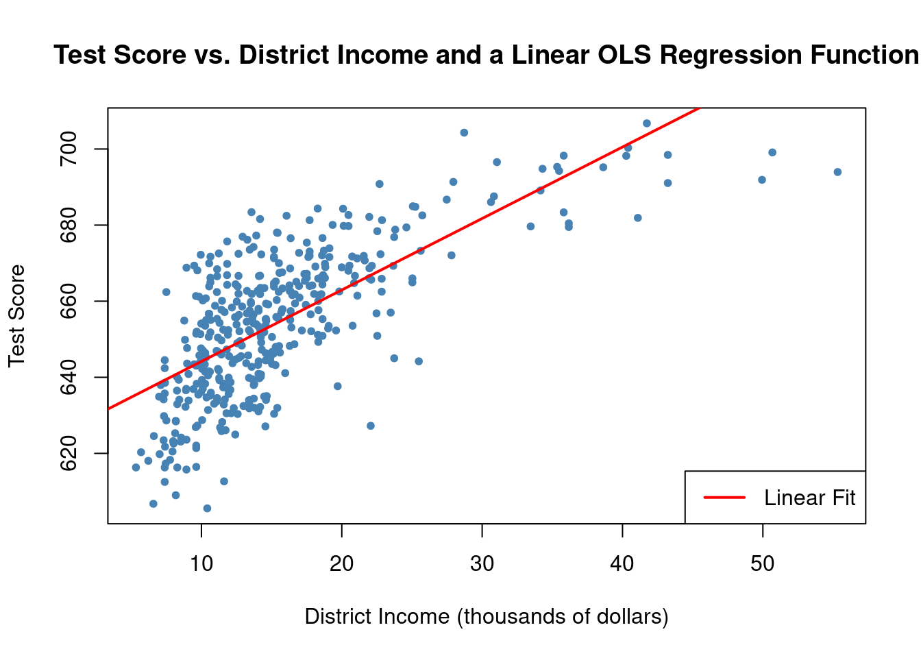
The plot shows that the linear regression line seems to overestimate the true relationship when income is either very high or very low and it tends to underestimates it for the middle income group. Luckily, Ordinary Least Squares (OLS) isn’t limited to linear regressions of the predictors. We have the flexibility to model test scores as a function of income and the square of income.
This leads us to the following regression model:
TestScore_i = \beta_0 + \beta_1 \, income_i + \beta_2 \, income_i^2 + u_i which is a quadratic regression model. Here we treat income^2 as an additional explanatory variable.
# fit the quadratic Model
quadratic_model <- lm(score ~ income + I(income^2), data = CASchools)

# obtain the model summary
coeftest(quadratic_model, vcov. = vcovHC)
t test of coefficients:

               Estimate  Std. Error  t value  Pr(>|t|)
(Intercept) 607.3017435   2.9242237 207.6796 < 2.2e-16 ***
income        3.8509939   0.2711045  14.2048 < 2.2e-16 ***
I(income^2)  -0.0423084   0.0048809  -8.6681 < 2.2e-16 ***
---
Signif. codes:  0 '***' 0.001 '**' 0.01 '*' 0.05 '.' 0.1 ' ' 1
The estimated function is
\widehat{TestScore} = \underset{(2.93)}{607.3} \,+ \underset{(0.27)}{3.85} \, income_i - \underset{(0.00489)}{0.0423} \, income_i^2
We will now draw the same scatter plot as for the linear model and add the regression line for the quadratic model. Since abline() only plots straight lines, it cannot be used here, but we can use lines() function instead, which is suitable for plotting nonstraight lines (see ?lines). The most basic call of lines() is lines(x_values, y_values) where x_values and y_values are vectors of the same length that provide coordinates of the points to be sequentially connected by a line.
This requires sorted coordinate pairs according to the X-values. We may use the function order() to sort the fitted values of score according to the observations of income, obtained from our quadratic model.
# Plot observations and add linear and quadratic regression lines
plot(CASchools$income, CASchools$score, col="steelblue", pch=20,
     xlab="District Income (thousands of dollars)", ylab="Test Score",
     main="Estimated Linear and Quadratic Regression Functions")
# Linear regression line
abline(linear_model, col="green", lwd=2)
# Quadratic regression line
lines(CASchools$income[order(CASchools$income)],
      fitted(quadratic_model)[order(CASchools$income)], col="red", lwd=2)
legend("bottomright", c("Quadratic Fit", "Linear Fit"), lwd=2, col=c("red", "green"))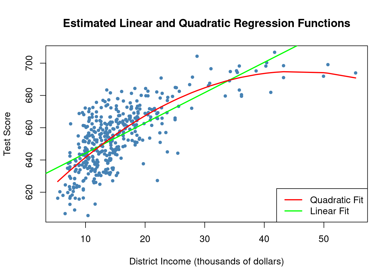
As the plot shows, the quadratic function appears to provide a better fit to the data compared to the linear function.
Another approach to estimate a concave nonlinear regression function involves using a logarithmic regressor.
# estimate a level-log model
LinearLog_model <- lm(score ~ log(income), data = CASchools)

# compute robust summary
coeftest(LinearLog_model, vcov = vcovHC)
t test of coefficients:

            Estimate Std. Error t value  Pr(>|t|)
(Intercept) 557.8323     3.8622 144.433 < 2.2e-16 ***
log(income)  36.4197     1.4058  25.906 < 2.2e-16 ***
---
Signif. codes:  0 '***' 0.001 '**' 0.01 '*' 0.05 '.' 0.1 ' ' 1
The estimated regression model is
\widehat{TestScore} = \underset{(3.86)}{557.8} + \underset{(1.41)}{36.42} \, \log (income)
We plot this function
# Draw a scatterplot with linear and linear-log regression lines
plot(score ~ income, data = CASchools, col = "steelblue", pch = 20,
     ylab="Score", xlab="Income", main = "Linear-Log Regression Line")
order_id <- order(CASchools$income)
# Linear-log regression line
lines(CASchools$income[order_id], fitted(LinearLog_model)[order_id],
      col = "red", lwd = 2)
# Linear regression line
lines(CASchools$income[order_id], fitted(linear_model)[order_id],
      col = "green", lwd = 2)
legend("bottomright", c("Linear-log Fit", "Linear Fit"),
       lwd = 2, col = c("red", "green"))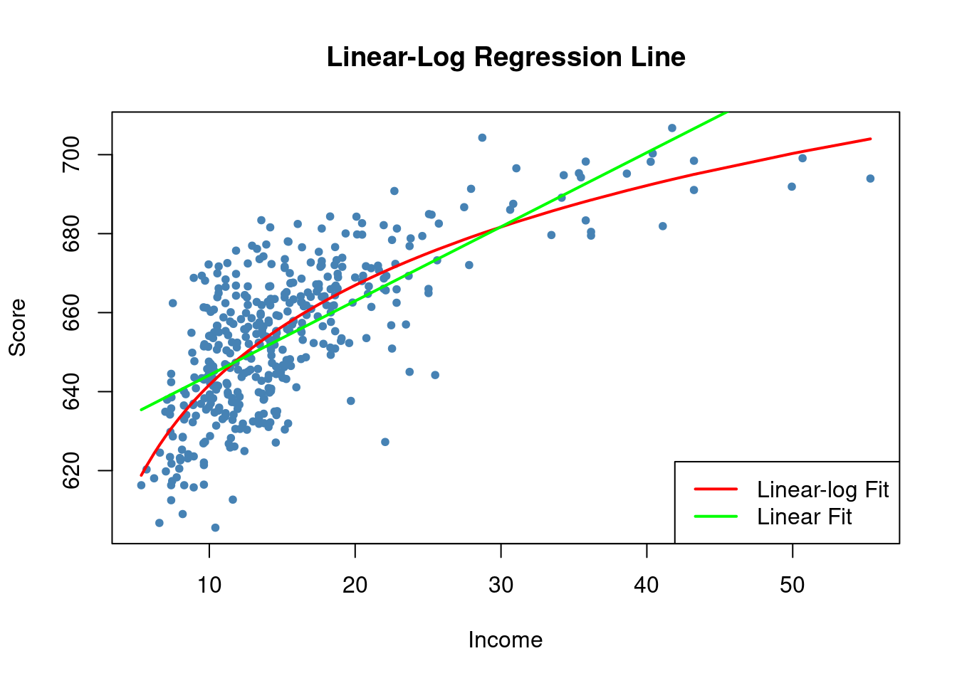
We can interpret \hat \beta_1 as follows: a 1\% increase in income is associated with an average increase in test scores of 0.01 \cdot 36.42 = 0.36 points.
6.6 Interactions
Sometimes it is interesting to learn how the effect on Y of a change in an independent variable depends on the value of another independent variable.
For example, we may ask if districts with many English learners benefit differently from a decrease in the student-teacher ratio compared to those with fewer English learning students. We can assess this by using a multiple regression model and including an interaction term.
We consider three cases: when both independent variables are binary, when one is binary and the other is continuous, and when both are continuous.
6.6.1 Two Binary Variables
Let HiSTR = \begin{cases} 1, & \text{if } \text{STR} \geq 20, \\ 0, & \text{else,} \end{cases} \quad HiEL = \begin{cases} 1, & \text{if } \text{english} \geq 10, \\ 0, & \text{else.} \end{cases} In R, we construct these dummies as follows
# append HiSTR to CASchools
CASchools$HiSTR <- as.numeric(CASchools$STR >= 20)

# append HiEL to CASchools
CASchools$HiEL <- as.numeric(CASchools$english >= 10)
We now estimate the model
TestScore = \beta_0 + \beta_1 \, HiSTR + \beta_2 \, HiEL + \beta_3 \, HiSTR \cdot HiEL + u_i.
We can simply indicate HiEL * HiSTR inside the lm() formula to add the interaction term to the model. Note that this adds HiEL, HiSTR and their interaction as regressors, whereas indicating HiEL:HiSTR only adds the interaction term.
# estimate the model with a binary interaction term
bi_model <- lm(score ~ HiSTR * HiEL, data = CASchools)

# print a robust summary of the coefficients
coeftest(bi_model, vcov. = vcovHC)
t test of coefficients:

            Estimate Std. Error  t value  Pr(>|t|)
(Intercept) 664.1433     1.3908 477.5272 < 2.2e-16 ***
HiSTR        -1.9078     1.9416  -0.9826    0.3264
HiEL        -18.3155     2.3453  -7.8094 4.721e-14 ***
HiSTR:HiEL   -3.2601     3.1360  -1.0396    0.2991
---
Signif. codes:  0 '***' 0.001 '**' 0.01 '*' 0.05 '.' 0.1 ' ' 1
The estimated regression model is
\widehat{TestScore} = \underset{(1.39)}{664.1} - \underset{(1.94)}{1.9} \, \text{HiSTR} - \underset{(2.35)}{18.3} \, \text{HiEL} - \underset{(3.14)}{3.3} \, (\text{HiSTR} \cdot \text{HiEL})
According to this model, when moving from a school district with a low student-teacher ratio to one with a high ratio, the average effect on test scores depends on the percentage of English learners (HiEL), and can be computed as -1.9 - 3.3 \cdot HiEL.
This is, for districts with fewer English learners (HiEL = 0), the expected decrease in test scores is 1.9 points. However, for districts with a higher proportion of English learners (HiEL = 1), the predicted decrease in test scores is 1.9 + 3.3 = 5.2 points.
We can estimate the mean test score conditional on all possible combination of the included binary variables
| HiSTR | HiEL | E[score | HiSTR, HiEL] | \widehat{score} |
|---|---|---|---|
| 0 | 0 | \beta_0 | 664.1 |
| 0 | 1 | \beta_0 + \beta_2 | 645.8 |
| 1 | 0 | \beta_0 + \beta_1 | 662.2 |
| 1 | 1 | \beta_0 + \beta_1 + \beta_2 + \beta_3 | 640.6 |
6.6.2 Continuous and Binary Variables
This specification where the interaction term includes a continuous variable (X_i) and a binary variable (D_i) allows for the slope to depend on the binary variable. There are three different possibilities:
- Different intercepts, same slope:
Y_i = \beta_0 + \beta_1 X_i + \beta_2 D_i + u_i
- Different intercepts and slopes:
Y_i = \beta_0 + \beta_1 X_i + \beta_2 D_i + \beta_3 (X_i \cdot D_i) + u_i
- Same intercept, different slopes:
Y_i = \beta_0 + \beta_1 X_i + \beta_2 (X_i \cdot D_i) + u_i. Does the effect on test scores of cutting the student-teacher ratio depend on whether the percentage of students still learning English is high or low?
One way to answer this question is to use a specification that allows for two different regression lines, depending on whether there is a high or a low percentage of English learners. This is achieved using the different intercept/different slope specification. We estimate the regression model
\widehat{TestScore}_i = \beta_0 + \beta_1 \, STR_i + \beta_2 \, HiEL_i + \beta_3 \, (STR_i \cdot HiEL_i) + u_i
# estimate the model
bci_model <- lm(score ~ STR + HiEL + STR * HiEL, data = CASchools)

# print robust summary of coefficients
coeftest(bci_model, vcov. = vcovHC)
t test of coefficients:

             Estimate Std. Error t value Pr(>|t|)
(Intercept) 682.24584   12.07126 56.5182   <2e-16 ***
STR          -0.96846    0.59943 -1.6156   0.1069
HiEL          5.63914   19.88866  0.2835   0.7769
STR:HiEL     -1.27661    0.98557 -1.2953   0.1959
---
Signif. codes:  0 '***' 0.001 '**' 0.01 '*' 0.05 '.' 0.1 ' ' 1
\widehat{TestScore} = \underset{(12.07)}{682.2} - \underset{(0.60)}{0.97} \, STR + \underset{(19.89)}{5.6} \, HiEL - \underset{(0.99)}{1.28} \, (STR \cdot HiEL).
The estimated regression line for districts with a low fraction of English learners (HiEL=0) is
\widehat{TestScore} = 682.2 - 0.97 \, STR_i while the one for districts with a high fraction of English learners (HiEL=1) is
\begin{align*} \widehat{TestScore} &= 682.2 + 5.6 - 0.97 \, STR_i - 1.28 \, STR_i \\ &= 687.8 - 2.25 \, STR_i. \end{align*}
The expected rise in test scores after decreasing the student-teacher ratio by one unit is roughly 0.97 points in districts with a low proportion of English learners, but 2.25 points in districts with a high concentration of English learners.
The coefficient on the interaction term, “STR \cdot HiEL”, indicates that the contrast between these effects amounts to 1.28 points.
We now plot both regression lines from the model by using different colors to differentiate each of the STR levels.
# Determine observations with English learners >= 10%
id <- CASchools$english >= 10

# Plot observations with different colors for HiEL status and draw regression lines
plot(CASchools$STR, CASchools$score, xlim = c(0, 27), ylim = c(600, 720), pch = 20,
     col = ifelse(id, "green", "red"), xlab = "Class Size", ylab = "Test Score")
legend("topleft", pch = 20, col = c("red", "green"), legend = c("HiEL = 0", "HiEL = 1"))
abline(coef = c(bci_model$coefficients[1], bci_model$coefficients[2]),
       col = "red", lwd = 1.5)
abline(coef = c(bci_model$coefficients[1] + bci_model$coefficients[3],
                bci_model$coefficients[2] + bci_model$coefficients[4]),
       col = "green", lwd = 1.5)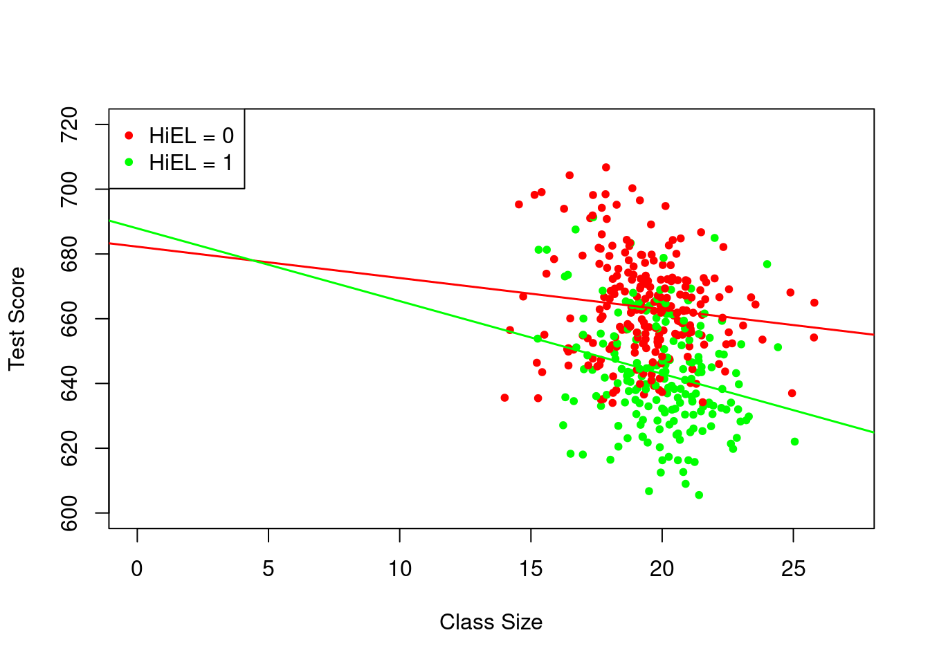
6.6.3 Two Continuous Variables
Let’s now examine the interaction between the continuous variables student-teacher ratio (STR) and the percentage of English learners (english).
# estimate regression model including the interaction between 'english' and 'STR'
cci_model <- lm(score ~ STR + english + english * STR, data = CASchools)

# print summary
coeftest(cci_model, vcov. = vcovHC)
t test of coefficients:

               Estimate  Std. Error t value Pr(>|t|)
(Intercept) 686.3385268  11.9378561 57.4926  < 2e-16 ***
STR          -1.1170184   0.5965151 -1.8726  0.06183 .
english      -0.6729119   0.3865378 -1.7409  0.08245 .
STR:english   0.0011618   0.0191576  0.0606  0.95167
---
Signif. codes:  0 '***' 0.001 '**' 0.01 '*' 0.05 '.' 0.1 ' ' 1
The estimated regression function is
\widehat{TestScore} = \underset{(11.94)}{686.3} - \underset{(0.60)}{1.12} \, STR - \underset{(0.39)}{0.67} \, english + \underset{(0.02)}{0.0012} \, (STR \cdot english).
Before proceeding with the interpretations, let us explore the quartiles of english
summary(CASchools$english) Min. 1st Qu. Median Mean 3rd Qu. Max.
0.000 1.941 8.778 15.768 22.970 85.540 When the percentage of English learners is at the median (english = 8.778), the slope of the line is estimated to be (-1.12 + 0.0012 \cdot 8.778 = -1.12). When the percentage of English learners is at the 75th percentile (english = 22.97), this line is estimated to be slightly flatter, with a slope of -1.12 + 0.0012 \cdot 22.97 = -1.09.
In other words, for a district with 8.78\% English learners, the estimated effect of a one-unit reduction in the student-teacher ratio is to increase on average test scores by 1.11 points, but for a district with 23\% English learners, reducing the student-teacher ratio by one unit is predicted to increase test scores on average by 1.09 points.
However, it is important to note from the output of coeftest() that the estimated coefficient on the interaction term (\beta_3) is not statistically significant at the 10\% level, so we cannot reject the null hypothesis H_0: \beta_3 = 0.
6.7 Nonliearities in Score Regressions
This section examines three key questions about test scores and the student-teacher ratio.
First, it explores if reducing the student-teacher ratio affects test scores differently based on the number of English learners, even when considering economic differences across districts.
Second, it investigates if this effect varies depending on the student-teacher ratio.
Lastly, it aims to determine the expected impact on test scores when the student-teacher ratio decreases by two students per teacher, considering both economic factors and potential nonlinear relationships.
We will answer these questions considering the previously explained nonlinear regression specifications, extended to include two measures of the economic background of the students: the percentage of students eligible for a subsidized lunch (lunch) and the logarithm of average district income (log(income)).
The logarithm of district income is used following our previous empirical analysis, which suggested that this specification captures the nonlinear relationship between scores and income.
We leave out the expenditure per pupil (expenditure) from our analysis because including it would suggest that spending changes with the student-teacher ratio (in other words, we would not be holding expenditures per pupil constant).
We will consider 7 different model specifications:
# estimate all models
TS_mod1 <- lm(score ~ STR + english + lunch, data = CASchools)
TS_mod2 <- lm(score ~ STR + english + lunch + log(income), data = CASchools)
TS_mod3 <- lm(score ~ STR + HiEL + HiEL:STR, data = CASchools)
TS_mod4 <- lm(score ~ STR + HiEL + HiEL:STR + lunch + log(income), data = CASchools)
TS_mod5 <- lm(score ~ STR + I(STR^2) + I(STR^3) + HiEL + lunch + log(income),
              data = CASchools)
TS_mod6 <- lm(score ~ STR + I(STR^2) + I(STR^3) + HiEL + HiEL:STR + HiEL:I(STR^2) + HiEL:I(STR^3)
              + lunch + log(income), data = CASchools)
TS_mod7 <- lm(score ~ STR + I(STR^2) + I(STR^3) + english + lunch + log(income),
              data = CASchools)

# gather robust standard errors in a list
rob_se <- list(sqrt(diag(vcovHC(TS_mod1))),
               sqrt(diag(vcovHC(TS_mod2))),
               sqrt(diag(vcovHC(TS_mod3))),
               sqrt(diag(vcovHC(TS_mod4))),
               sqrt(diag(vcovHC(TS_mod5))),
               sqrt(diag(vcovHC(TS_mod6))),
sqrt(diag(vcovHC(TS_mod7))))stargazer(TS_mod1, TS_mod2, TS_mod3, TS_mod4,
TS_mod5, TS_mod6, TS_mod7,
se = rob_se,
type="html",
omit.stat = "f", df=FALSE)| Dependent variable: | |||||||
| score | |||||||
| (1) | (2) | (3) | (4) | (5) | (6) | (7) | |
| STR | -0.998*** | -0.734*** | -0.968 | -0.531 | 64.339** | 83.702*** | 65.285** |
| (0.274) | (0.261) | (0.599) | (0.350) | (27.295) | (31.506) | (27.708) | |
| english | -0.122*** | -0.176*** | -0.166*** | ||||
| (0.033) | (0.034) | (0.035) | |||||
| I(STR2) | -3.424** | -4.381*** | -3.466** | ||||
| (1.373) | (1.597) | (1.395) | |||||
| I(STR3) | 0.059*** | 0.075*** | 0.060*** | ||||
| (0.023) | (0.027) | (0.023) | |||||
| lunch | -0.547*** | -0.398*** | -0.411*** | -0.420*** | -0.418*** | -0.402*** | |
| (0.024) | (0.034) | (0.029) | (0.029) | (0.029) | (0.034) | ||
| log(income) | 11.569*** | 12.124*** | 11.748*** | 11.800*** | 11.509*** | ||
| (1.841) | (1.823) | (1.799) | (1.809) | (1.834) | |||
| HiEL | 5.639 | 5.498 | -5.474*** | 816.076** | |||
| (19.889) | (10.012) | (1.046) | (354.100) | ||||
| STR:HiEL | -1.277 | -0.578 | -123.282** | ||||
| (0.986) | (0.507) | (54.290) | |||||
| I(STR2):HiEL | 6.121** | ||||||
| (2.752) | |||||||
| I(STR3):HiEL | -0.101** | ||||||
| (0.046) | |||||||
| Constant | 700.150*** | 658.552*** | 682.246*** | 653.666*** | 252.050 | 122.353 | 244.809 |
| (5.641) | (8.749) | (12.071) | (10.053) | (179.724) | (205.050) | (181.899) | |
| Observations | 420 | 420 | 420 | 420 | 420 | 420 | 420 |
| R2 | 0.775 | 0.796 | 0.310 | 0.797 | 0.801 | 0.803 | 0.801 |
| Adjusted R2 | 0.773 | 0.794 | 0.305 | 0.795 | 0.798 | 0.799 | 0.798 |
| Residual Std. Error | 9.080 | 8.643 | 15.880 | 8.629 | 8.559 | 8.547 | 8.568 |
| Note: | p<0.1; p<0.05; p<0.01 | ||||||
What can be concluded from the results presented?
First, we we see the estimated coefficient on STR is highly significant in all models except from specifications (3) and (4).
When we add log(income) to model (1) in the second specification, all coefficients remain highly significant while the coefficient on the new regressor is also statistically significant at the 1\% level. Additionally, the coefficient on STR is now 0.27 higher than in model (1), suggesting a possible mitigation of omitted variable bias when including log(income) as regressor. For these reasons, it makes sense to keep this variable in other models too.
Models (3) and (4) include the interaction term between STR and HiEL, first without control variables in the third specification and then controlling for economic factors in the fourth. The estimated coefficient for the interaction term is not significant at any common level in any of these models, nor is the coefficient on the dummy variable HiEL. Hence, despite accounting for economic factors, we cannot reject the null hypotheses that the impact of the student-teacher ratio on test scores remains consistent across districts with high and low proportions of English learning students.
In regression (5) we have included quadratic and cubic terms for STR, while omitting the interaction term between STR and HiEL, since it was not significant in specification (4). The results indicate high levels of significance for these estimated coefficients and we can therefore assume the presence of a nonlinear effect of the student-teacher ration on test scores. This could be also verified with an F-test of H_0: \beta_2 = \beta_3 =0.
Regression (6) further examines whether the proportion of English learners influences the student-teacher ratio, incorporating the interaction terms HiEL\cdot STR, HiEL\cdot STR^2 and HiEL\cdot STR^3. Each individual t-test confirms significant effects. To validate this, we perform a robust F-test to assess H_0: \beta_5 = \beta_6 = \beta_7 =0.
# check joint significance of the interaction terms
waldtest(TS_mod6,
         c("STR:HiEL", "I(STR^2):HiEL", "I(STR^3):HiEL"),
         vcov = vcovHC)
Wald test
Model 1: score ~ STR + I(STR^2) + I(STR^3) + HiEL + HiEL:STR + HiEL:I(STR^2) +
HiEL:I(STR^3) + lunch + log(income)
Model 2: score ~ STR + I(STR^2) + I(STR^3) + HiEL + lunch + log(income)
Res.Df Df F Pr(>F)
1 410
2 413 -3 2.1885 0.08882 .
---
Signif. codes: 0 '***' 0.001 '**' 0.01 '*' 0.05 '.' 0.1 ' ' 1With a p-value of 0.08882 we can just reject the null hypothesis at the 10\% level. This provides only weak evidence that the regression functions are different for districts with high and low percentages of English learners.
In model (7), we employ a continuous measure for the proportion of English learners instead of a dummy variable (thus omitting interaction terms). We note minimal alterations in the coefficient estimates for the remaining regressors. Consequently, we infer that the findings observed in model (5) are robust and not influenced significantly by the method used to measure the percentage of English learners.
We can now address the initial questions raised in this section:
First, in the linear models, the impact of the percentage of English learners on changes in test scores due to variations in the student-teacher ratio is minimal, a conclusion that holds true even after accounting for students’ economic backgrounds. Although the cubic specification (6) suggests that the relationship between student-teacher ratio and test scores is influenced by the proportion of English learners, the magnitude of this influence is not significant.
Second, while controlling for students’ economic backgrounds, we identify nonlinearities in the association between student-teacher ratio and test scores.
Lastly, under the linear specification (2), a reduction of two students per teacher in the student-teacher ratio is projected to increase test scores by approximately 1.46 points. As this model is linear, this effect remains consistent regardless of class size. For instance, assuming a student-teacher ratio of 20, the nonlinear model (5) indicates that the reduction in student-teacher ratio would lead to an increase in test scores by \begin{align*} \small &64.33 \cdot 18 + 18^2 \cdot (-3.42) + 18^3 \cdot (0.059) \\ &\quad - (64.33 \cdot 20 + 20^2 \cdot (-3.42) + 20^3 \cdot (0.059)) \\ &\approx 3.3 \end{align*} points. If the ratio was 22, a reduction to 20 leads to a predicted improvement in test scores of \begin{align*} \small &64.33 \cdot 20 + 20^2 \cdot (-3.42) + 20^3 \cdot (0.059) \\ &\quad - (64.33 \cdot 22 + 22^2 \cdot (-3.42) + 22^3 \cdot (0.059)) \\ &\approx 2.4 \end{align*} points. This suggests that the effect is more evident in smaller classes.