13 Case Study III: Big Data
13.1 Introduction
In this case study, we will explore the empirical application of prediction methods using the test score data set from California elementary schools. The data set includes detailed information on various school and community characteristics, which allows us to experiment with different regression models and prediction techniques.
We aim to predict fifth-grade test scores using three different sets of predictors: a small set with only a few variables, a large set with many variables, and a very large set with an extensive number of predictors, including interactions, squares, and cubes of the main variables.
13.2 Data Set Description
The primary data set contains data on 3932 elementary schools in California from 2013. The raw data and its variable descriptions can be downloaded here (CA_Schools_EE14).
Data has been splitted into three sets based on the number of predictors:
- Small Data Set: Contains 4 variables that have been commonly used in previous studies:
Student-teacher ratio (
str_s)Median income of the local population (
med_income_z)Teachers average years of experience (
te_avgyr_s)Instructional expenditures per student (
exp_1000_1999_d)
Large Data Set: Contains 817 predictors including 38 main variables, their squares, cubes, and all possible pairwise interactions. The main variables cover student demographics, teacher characteristics, school funding, and expenditure metrics, including fractions of students by eligibility and ethnicity, teacher experience, school expenditures, and district-level financial data.
Very Large Data Set: Contains 2065 predictors, which includes additional demographic variables, their squares, cubes, and interactions with the binary variables describing school characteristics.
For simplicity, these data sets have been prepared for you and can be accessed directly from the xlsx files (see Ilias course):
data_large = read_xlsx("data_large.xlsx")We will use the large data set here, but you can apply the same code to the small and the very large data set.
Here you find a script to create your own data sets based on the raw data.
13.3 Methods
We will use four different methods to estimate the predictive models:
Ordinary Least Squares (OLS)
Ridge Regression
Lasso Regression
Principal Components Regression (PCR)
These methods will be applied to each of the data sets to evaluate their performance in predicting out-of-sample test scores. The main metric used to assess the prediction accuracy is the Root Mean Squared Error (RMSE).
13.4 Data Preparation
The data is processed and divided into training and test sets (50/50 split), with 1966 observations each. The predictor variables are standardized, and the response variable is the average fifth-grade test score at the school.
## Select the data set to be used (large dataset in this case)
mydata = data_large

## Split 50/50 into training and test sets
set.seed(123) #for reproducibility
train_indices = sample(1:nrow(mydata), size = 0.5*nrow(mydata))
train_data = mydata[train_indices, ]
test_data = mydata[-train_indices, ]

## Standardize/scale the predictor variables
train_response = train_data$testscore
train_predictors = train_data |> select(-testscore) |> scale()
test_response = test_data$testscore
test_predictors = test_data |> select(-testscore) |> scale()
13.5 Cross-Validation for Tuning Parameters
13.5.1 Ridge Regression
For ridge regression, we perform 10-fold cross-validation to select the optimal shrinkage parameter (\lambda). The tuning parameter that minimizes the cross-validated RMSE is chosen for the final model.
The train() function from the caret package can be used for cross validation. We set alpha to 0 for ridge regression and we try out different lambdas specified in the sequence given by lambdagrid.
# grid for lambdas over which to cross validate. the finer the grid, the longer it takes
lambdagrid = exp(seq(0,7,length=100))

cv.ridge = train(
  x=train_predictors,
  y=train_response,
  method = "glmnet",
  metric = "RMSE",
  tuneGrid = expand.grid(alpha = 0,lambda = lambdagrid),
  trControl = trainControl(method = "cv", number = 10) # 10-fold cv
)
plot(cv.ridge) # plot the cv results for ridge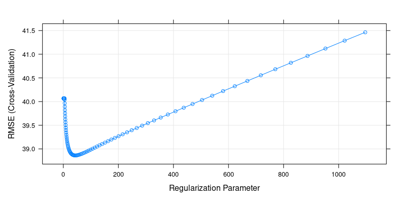
Cross-Validation Results for Ridge Regression
# print best tuning parameters for ridge
cv.ridge$bestTune
[1] 42.41384We can also fine-tune lambda in a specific region to get a better picture, e.g. around 30-50:
cv.ridge.finetune = train(
  x=train_predictors,
  y=train_response,
  method = "glmnet",
  metric = "RMSE",
  tuneGrid = expand.grid(alpha = 0,lambda = seq(30,50, length = 101)),
  trControl = trainControl(method = "cv", number = 10)
)
plot(cv.ridge.finetune)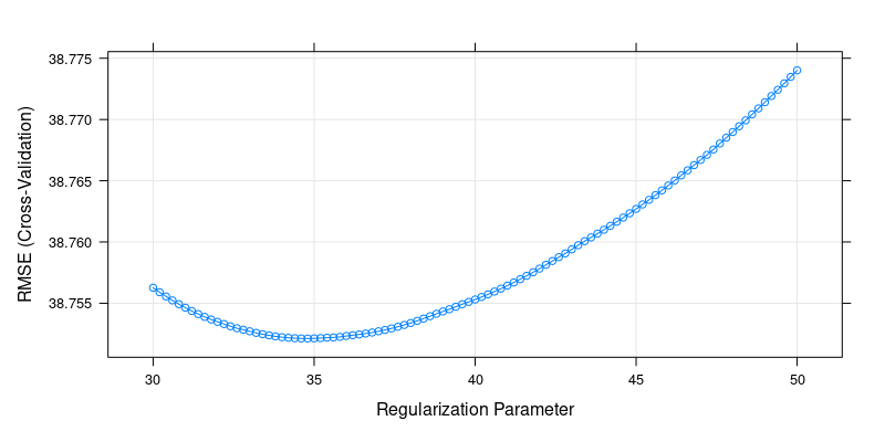
# the result may be slightly different each time because the folds are sampled randomly
cv.ridge.finetune$bestTune
[1] 34.8The built-in cross-validation method of the glmnet package gives a similar tuning parameter:
cv.ridge2 = cv.glmnet(x=train_predictors, y=train_response, alpha=0)
cv.ridge2$lambda.min
[1] 39.2749113.5.2 Lasso Regression
Similar to ridge regression, we use 10-fold cross-validation to find the optimal shrinkage parameter for the lasso model.
The procedure is the same, but now we set alpha = 1 for lasso.
lambdagrid = seq(0, 2, length = 101)

cv.lasso = train(
  x = train_predictors,
  y = train_response,
  method = "glmnet",
  metric = "RMSE",
  tuneGrid = expand.grid(alpha = 1, lambda = lambdagrid),
  trControl = trainControl(method = "cv", number = 10) # 10-fold cv
)
plot(cv.lasso)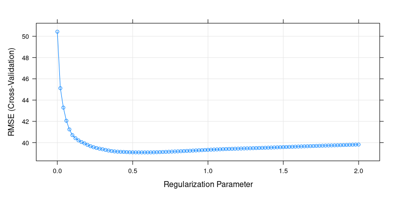
Cross-Validation Results for Lasso Regression
# print best tuning parameters for lasso
cv.lasso$bestTune
[1] 0.56Again, we can alternatively use the glmnet package with its built-in cross-validation method:
cv.lasso2 = cv.glmnet(x=train_predictors, y=train_response, alpha=1)
cv.lasso2$lambda.min
[1] 0.484199513.5.3 Principal Components Regression
For principal component regression (PCR), we use principal components analysis to determine the number of components that explain a significant amount of variance in the predictors. We then use 10-fold cross-validation to select the number of principal components that balances bias and variance for the regression model.
## Principal Component Analysis
pca_result = prcomp(train_predictors)
X_pca = pca_result$x # Full matrix of all principal component scores
We then use a subset of the principal components as predictors in a regression model. Here, we start by using the first four principal components.
## Run a PC-regression with ncomp=4 principal components
ncomp = 4
data_pca = data.frame(y = train_response, X_pca[, 1:ncomp])
lm(y~., data = data_pca)
Call:
lm(formula = y ~ ., data = data_pca)

Coefficients:
(Intercept)          PC1          PC2          PC3          PC4
    752.792       -2.480       -2.183        2.294        1.436
By regressing on the first few principal components, we reduce the dimensionality of the problem. This can help prevent overfitting, as the components capture the most important information from the original predictors while ignoring the noise.
To decide how many principal components to use, we can plot the scree plot, which shows the fraction of total variance explained by each principal component.
## Scree Plot: Fraction of variance explained
var_explained = pca_result$sdev^2 / sum(pca_result$sdev^2)
plot(var_explained[1:70], type="b",
     xlab = "Principal Component", ylab = "Fraction of Variance Explained")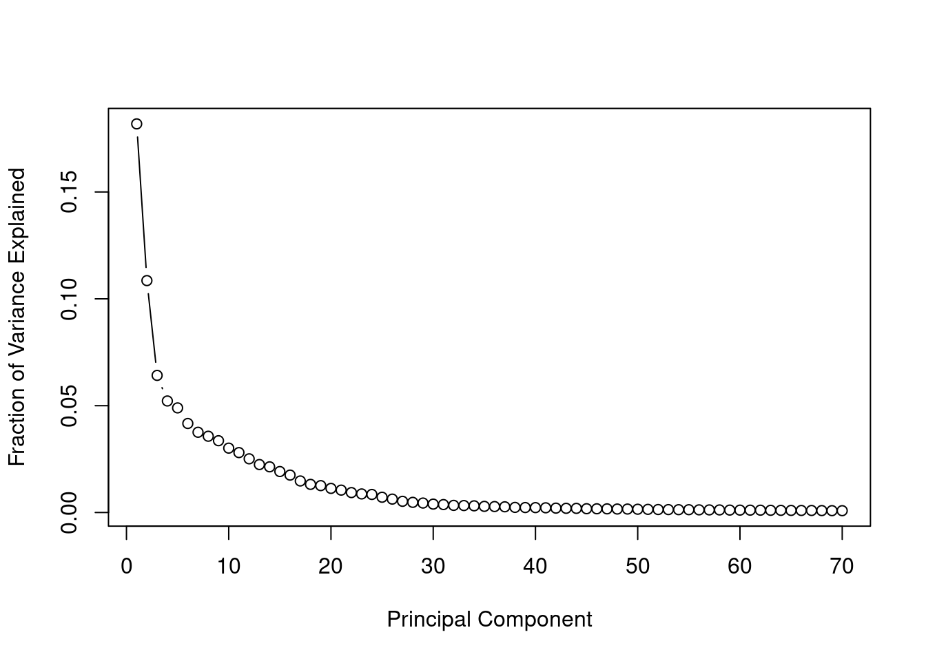
Scree Plot: Fraction of variance explained
The scree plot indicates an elbow around 30-40 components. We can also determine the number of principal components needed to explain a specific percentage of the total variance.
[1] 34[1] 62[1] 157Retaining components that explain 90%-95% of the variance is a common practice to ensure that most of the underlying structure of the data is preserved while omitting unnecessary noise.
Finally, we use cross-validation to find the optimal number of principal components that minimizes the mean squared prediction error.
## PCR 10-fold cross-validation
myfunc.cvpca = function(p){
  data_pca = data.frame(y = train_response, X_pca[,1:p])
  cv = train(
    y ~ ., data = data_pca,
    method = "lm",
    metric = "RMSE",
    trControl = trainControl(method = "cv", number = 10)
  )
  return(cv$results$RMSE)
}
# Iterate function crossval over ncomp = 1, ..., maxcomp
maxcomp = 150 # select not more than number of variables (for data_small select <=4)
cv.pca = sapply(1:maxcomp, myfunc.cvpca) # sapply is useful for iterating over function arguments ncomp

# Find the number of components with the lowest RMSPE
which.min(cv.pca)
plot(cv.pca, type="l")
[1] 48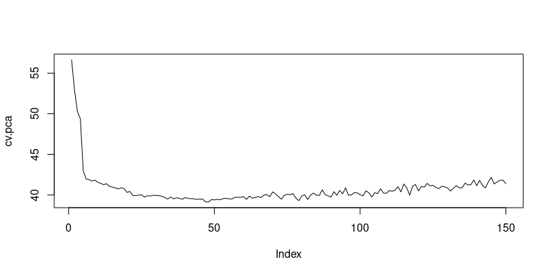
Cross-Validation Results for Principal Components Regression
13.6 Summary
We can now summarize the tuning parameters that were determined through cross-validation for each predictive method and each data set.
Estimated \lambda or p:
| Data Set | Ridge | Lasso | PCR |
|---|---|---|---|
| Small (k = 4) | 3.33 | 0.4 | 4 |
| Large (k = 817) | 42.41 | 0.56 | 48 |
| Very Large (k = 2065) | 437.38 | 0.58 | 73 |
The parameters are selected by minimizing the MSPE through 10-fold cross-validation using the 1966 observations in the training sample.
We reserved a separate test sample of 1966 observations, independent of the training sample. To evaluate the predictive performance, we use the estimated models from the training sample to predict Y_i from \boldsymbol{X_i} for all i in the test sample and then assess the mean prediction errors. As a baseline competitor, we include the OLS predictor.
## OLS
fit.ols = lm(testscore ~., data = train_data)
oospred.ols = predict(fit.ols, newdata = test_data)

## Ridge
lambda.ridge = 42.41
fit.ridge = glmnet(x=train_predictors, y=train_response, alpha=0, lambda = lambda.ridge)
oospred.ridge = predict(fit.ridge, test_predictors)

## LASSO
lambda.lasso = 0.56
fit.lasso = glmnet(x=train_predictors, y=train_response, alpha=1, lambda = lambda.lasso)
oospred.lasso = predict(fit.lasso, test_predictors)

## PCA
p.pcr = 48
pca_result = prcomp(train_predictors)
data_pca = data.frame(y=train_response, pca_result$x[,1:p.pcr])
fit.pcr = lm(y~., data = data_pca)
## Estimated principal component weights
w = pca_result$rotation
## Principal components for the training data (coincides with pca_result$x):
P.train = train_predictors %*% w
##  Principal components for the test data:
P.test = test_predictors %*% w
datapca.test = data.frame(y=test_response, P.test[,1:p.pcr])
## out of sample prediction
oospred.pca = predict(fit.pcr, newdata = datapca.test)[1] 61.8867[1] 39.10138[1] 39.33968[1] 39.82125We can now present all out-of-sample MSPEs for all data sets in a summary table. We select the tuning parameters \lambda and p from the table above.
| Data Set | OLS | Ridge | Lasso | PCR |
|---|---|---|---|---|
| Small | 52.44 | 52.47 | 52.45 | 52.48 |
| Large | 61.89 | 39.1 | 39.34 | 39.82 |
| Very Large | - | 39.39 | 39.42 | 39.95 |
OLS is infeasible in the very large dataset because k > n. Ridge, lasso, and PCR perform similarly well, in particular in the large and the very large data set.